 The Dawn of Man. Image Credit: Movie Mezannine
Wyoming INBRE Bioinformatics Core
Dept. of Molecular Biology
University of Wyoming
The Dawn of Man. Image Credit: Movie Mezannine
1. Put away your phone for the duration of the class
2. Do not race ahead in the tutorial.
3. Doing so compromises your learning experience.
4. You may not leave early today!
For this entire exercise, replace <inbreNNN> with your own inbre ID. Once you log onto the Teton computing environment, copy the data for today’s exercise as follows.
$ ssh <inbreNNN>@teton.uwyo.edu

$ cd /project/inbre-train/<inbreNNN>/

$ mkdir Week5_LastName && cd Week5_LastName/

$ cp -r /project/inbre-train/Week5Data/* .

$ ls -lh
This is a standard format for storing information on polymorphism across the genome. It is a n x n matrix of individuals and variants. Columns refer to individuals, whereas rows refer to variants (SNPs). Analogous to the FASTQ format, VCF also stores quality information. Files formatted to store variant calls always end in .vcf extension. For example: input.vcf. The VCF format specification is described in detail in the user manual available at http://samtools.github.io.
VCFTools is a program that can parse and manipulate the information in .vcf files. A comprehensive user manual on VCFTools usage is available here. Before we can use this program, we must load it in memory as a module.
module load gcc swset

module load vcftools

vcftools

VCFtools (0.1.14)
© Adam Auton and Anthony Marcketta 2009

Process Variant Call Format files

For a list of options, please go to:
    https://vcftools.github.io/man_latest.html

Alternatively, a man page is available, type:
    man vcftools

Questions, comments, and suggestions should be emailed to:
    vcftools-help@lists.sourceforge.net
We have provided you with an example .vcf file for today’s exercise: human_chr15.vcf. As the name suggests, this file contains data from Homo sapiens Chromosome 15. The data was collected as part of the 1000 Genomes Project whose aim is to understand human genomic variation across the globe. This data is from the final phase of the project and contains genotypes of over 2500 individuals from 26 populations distributed globally genotyped at more than 84 million SNPs. See the map below for where those populations come from:
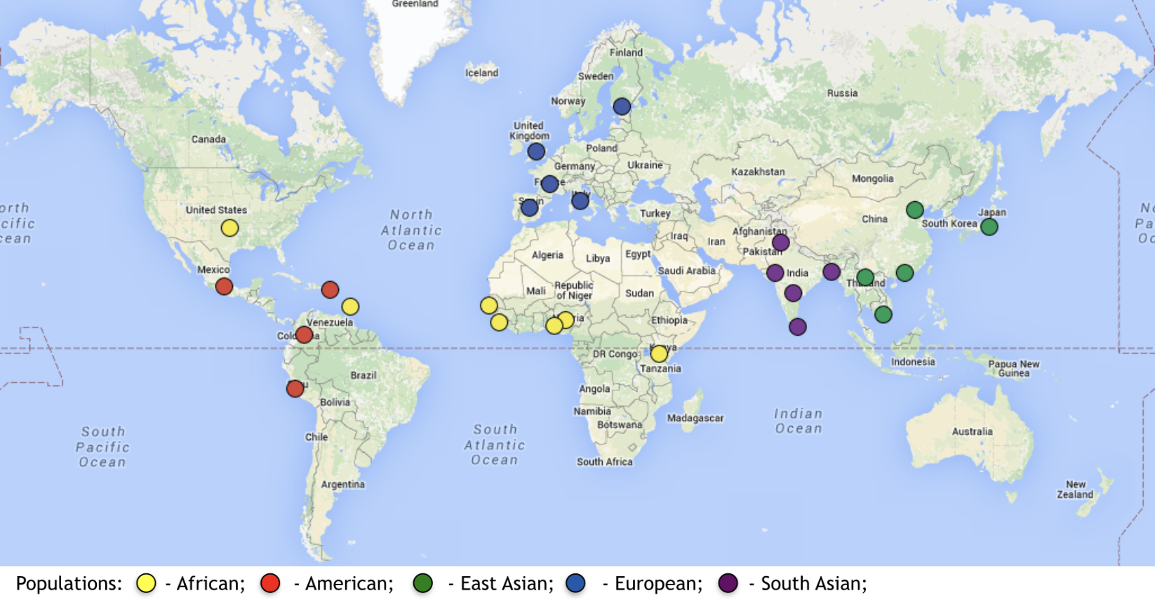 Image Credit: 1000 Genomes Project
To make it more manageable, we have subset the original data to only include information on 16000 SNPs. You will be further subsetting this file to obtain data on one specific SNP that we are interested in. But for now, open the file in text editor and take a look at the contents. Then close the file without saving.
Note: vi that you have been using so far is synonymous with vim. Both commands work the same.
VCFTools can provide a quick summary of your data. When running without any options, VCFTools outputs summary statistics but does not make any changes to the file nor does it produce any output files.
vcftools --vcf human_chr15.vcf

VCFtools - 0.1.14
(C) Adam Auton and Anthony Marcketta 2009

Parameters as interpreted:
    --vcf human_chr15.vcf

After filtering, kept 2504 out of 2504 Individuals
After filtering, kept 16003 out of a possible 16003 Sites
Run Time = 1.00 secondsrs1426654For today’s exercise, we are interested in only one SNP: rs1426654. Every documented SNP from the human genome has a rs ID associated with it. Note that the number following rs, is not the physical position of this SNP on a chromosome, but simply an identifier. You can look up the physical position of this SNP in the VCF file. For example:
Why did we pass the output of grep to cut via a |? It’s because when grep matches a pattern, it prints the entire line to the screen. Our lines here have more than 2500 columns and at this time, we are only interested in the first few columns as displayed above.
The gene SLC24A5 encodes a protein called Na/K/Ca Exchanger 5 which greatly influences skin color in humans. The leading hypothesis is that when our ancestors traveled out of Africa into Europe, the darker skin color was of no advantage in Europe’s cold climate. So eventually a new variant of the gene evolved in northern human populations which reduced the amount of skin pigmentation. By comparing the frequency of the two forms (alleles) of this gene in various human populations, we can study how populations can adapt differently when they are subject to very different environments.
rs1426654While there are more than 16,000 SNPs in our vcf file, we only need one for today’s exercise. So let’s go ahead and subset the VCF for that SNP.
vcftools --vcf human_chr15.vcf --snp rs1426654 --recode --out SLC24A5


VCFtools - 0.1.14
(C) Adam Auton and Anthony Marcketta 2009

Parameters as interpreted:
    --vcf human_chr15.vcf
    --out SLC24A5
    --recode
    --snp rs1426654

After filtering, kept 2504 out of 2504 Individuals
Outputting VCF file...
After filtering, kept 1 out of a possible 16003 Sites
Run Time = 1.00 seconds
In the above command, we extracted data for SNP rs1426654 from the file human_chr15.vcf and provided a prefix SLC24A5 for the output file. Check the output:
ls -lh

-rw-rw-r-- 1 vchhatre inbre-train 156M Nov  5 21:44 human_chr15.vcf
-rw-rw-r-- 1 vchhatre inbre-train  307 Nov  5 22:54 SLC24A5.log
-rw-rw-r-- 1 vchhatre inbre-train  30K Nov  5 22:54 SLC24A5.recode.vcf
The information that was printed to the screen was also populated inside the log file SLC24A5.log. Your main output file is SLC24A5.recode.vcf, but let’s change its name to SLC24A5.vcf for convenience.
$ mv SLC24A5.recode.vcf SLC24A5.vcf

$ ls -lh

-rw-rw-r-- 1 vchhatre inbre-train 30K Nov 5 22:54 SLC24A5.recode.vcfAs we discussed earlier, allele frequency is a measure of the relative proportion of the two (sometimes more) forms of a gene in a population. If a given SNP is not polymorphic, it will have only one allele (form). Frequency of that form will be f = 1.00 or 100%. However, if it is polymorphic, the resulting gene forms (alleles) may be present at any frquency from 0.01 to 0.99, whereas the other allele’s frequency will then be proportionately between 0.99 and 0.1. No matter their relative proportion, the frequencies of the two alleles will always add up to 1 in any population sample.
rs1426654 AllelesWe can use VCFTools to quickly estimate frequencies of the two alleles (A/G). But remember that allele frequency is a measure of population(s). During today’s exercise, we want to calculate these frequencies in each of the 26 human populations that we have data for. However, the vcf files does not contain any information on which individuals belong to which populations. Instead the population classification information is present in the folder popfiles:
$ ls -lh popfiles/
total 0

-rw-r--r-- 1 vchhatre  792 Nov  5 21:55 ESN.pop
-rw-r--r-- 1 vchhatre  816 Nov  5 21:55 STU.pop
-rw-r--r-- 1 vchhatre  768 Nov  5 21:55 PJL.pop
-rw-r--r-- 1 vchhatre  856 Nov  5 21:55 IBS.pop
-rw-r--r-- 1 vchhatre  744 Nov  5 21:55 CDX.pop
-rw-r--r-- 1 vchhatre  752 Nov  5 21:55 CLM.pop
-rw-r--r-- 1 vchhatre  512 Nov  5 21:55 MXL.pop
-rw-r--r-- 1 vchhatre  824 Nov  5 21:55 CHB.pop
-rw-r--r-- 1 vchhatre  832 Nov  5 21:55 PUR.pop
-rw-r--r-- 1 vchhatre  792 Nov  5 21:55 KHV.pop
-rw-r--r-- 1 vchhatre  824 Nov  5 21:55 GIH.pop
-rw-r--r-- 1 vchhatre  680 Nov  5 21:55 PEL.pop
-rw-r--r-- 1 vchhatre  728 Nov  5 21:55 GBR.pop
-rw-r--r-- 1 vchhatre  856 Nov  5 21:55 TSI.pop
-rw-r--r-- 1 vchhatre  792 Nov  5 21:55 LWK.pop
-rw-r--r-- 1 vchhatre  680 Nov  5 21:55 MSL.pop
-rw-r--r-- 1 vchhatre  688 Nov  5 21:55 BEB.pop
-rw-r--r-- 1 vchhatre  864 Nov  5 21:55 YRI.pop
-rw-r--r-- 1 vchhatre  840 Nov  5 21:55 CHS.pop
-rw-r--r-- 1 vchhatre  816 Nov  5 21:55 ITU.pop
-rw-r--r-- 1 vchhatre  792 Nov  5 21:55 FIN.pop
-rw-r--r-- 1 vchhatre  832 Nov  5 21:55 JPT.pop
-rw-r--r-- 1 vchhatre  488 Nov  5 21:55 ASW.pop
-rw-r--r-- 1 vchhatre  792 Nov  5 21:55 CEU.pop
-rw-r--r-- 1 vchhatre  904 Nov  5 21:55 GWD.pop
-rw-r--r-- 1 vchhatre  768 Nov  5 21:55 ACB.pop
Each of these popfiles contains a list of individuals that belong to that specific population. Try using the linux command cat on some of the files to see what is inside. You will notice that number of lines in each file corresponds to the number of individuals in it, with one individual listed per line.
Next, we will be writing a simple shell script to automate the estimation of allele frequencies using these population files and VCFTools. This script consumes very little computational resources, so we will not run it using sbatch. Thus you can exclude the scheduler commands that begin with #SBATCH for this script.
vim makefreq.sh

   #!/bin/bash

   ## First load the modules
   module load gcc swset vcftools

   ## Move to the appropriate directory
   cd /project/inbre-train/<inbreNNN>/Week5_LastName/

   ## Make folder to store frequency output
   mkdir freq

   ## Navigate to the folder ‘popfiles/’
   cd popfiles/

   ## For loop
   for p in *.pop
   do
     vcftools --vcf ../SLC24A5.vcf --keep $p --freq --out ../freq/$p
   done
   cd ..
Save and close the file. This script demonstrates a simple for loop which iterates over popfiles shown above and executes vcftools (to estimate allele frequencies) for only the individuals in the population file currently under iteration (Think back to our example of two populations during the lecture). Go ahead and execute it. Then look at the results.
bash makefreq.sh  ## Note, it is 'bash', not 'sbatch'.

pwd
/project/inbre-train/<inbreNNN>/Week5_LastName

cd freq

ls -othr *.frq

-rw-rw-r-- 1 vchhatre 80 Oct 28 23:55 ACB.pop.frq
-rw-rw-r-- 1 vchhatre 80 Oct 28 23:55 ASW.pop.frq
-rw-rw-r-- 1 vchhatre 80 Oct 28 23:55 BEB.pop.frq
-rw-rw-r-- 1 vchhatre 66 Oct 28 23:55 CDX.pop.frq
-rw-rw-r-- 1 vchhatre 66 Oct 28 23:55 CEU.pop.frq
-rw-rw-r-- 1 vchhatre 81 Oct 28 23:55 CHB.pop.frq
-rw-rw-r-- 1 vchhatre 81 Oct 28 23:55 CHS.pop.frq
-rw-rw-r-- 1 vchhatre 80 Oct 28 23:55 CLM.pop.frq
-rw-rw-r-- 1 vchhatre 81 Oct 28 23:55 ESN.pop.frq
-rw-rw-r-- 1 vchhatre 80 Oct 28 23:55 FIN.pop.frq
-rw-rw-r-- 1 vchhatre 66 Oct 28 23:55 GBR.pop.frq
-rw-rw-r-- 1 vchhatre 81 Oct 28 23:55 GIH.pop.frq
-rw-rw-r-- 1 vchhatre 81 Oct 28 23:55 GWD.pop.frq
-rw-rw-r-- 1 vchhatre 66 Oct 28 23:55 IBS.pop.frq
-rw-rw-r-- 1 vchhatre 80 Oct 28 23:55 ITU.pop.frq
-rw-rw-r-- 1 vchhatre 82 Oct 28 23:55 JPT.pop.frq
-rw-rw-r-- 1 vchhatre 82 Oct 28 23:55 KHV.pop.frq
-rw-rw-r-- 1 vchhatre 81 Oct 28 23:55 LWK.pop.frq
-rw-rw-r-- 1 vchhatre 81 Oct 28 23:55 MSL.pop.frq
-rw-rw-r-- 1 vchhatre 80 Oct 28 23:55 MXL.pop.frq
-rw-rw-r-- 1 vchhatre 80 Oct 28 23:55 PEL.pop.frq
-rw-rw-r-- 1 vchhatre 78 Oct 28 23:55 PJL.pop.frq
-rw-rw-r-- 1 vchhatre 80 Oct 28 23:55 PUR.pop.frq
-rw-rw-r-- 1 vchhatre 80 Oct 28 23:55 STU.pop.frq
-rw-rw-r-- 1 vchhatre 81 Oct 28 23:55 TSI.pop.frq
-rw-rw-r-- 1 vchhatre 81 Oct 28 23:55 YRI.pop.frq
Above, we have truncated the output of the ls command to only include files whose names end in .frq. There are however 52 files in the freq/ folder, of which half are .frq files and the other half are .log files from VCFTools. Let’s look inside one of the population allele frequency files.
The output is self explanatory. The SNP we are studying (rs1426654) is located on Chromosome 15 at base position 48426484. Being polymorphic, it has two forms (alleles). In population LWK, there are 198 chromosomes altogether (2 homologs per individual @ 99 individuals). Finally, frequencies of both alleles are provided. Notice that the frequencies add up to 1.0 as per expectation.
In order to visualize these allele frequencies for all 26 populations, we first need to combine information from all 26 output files. Simplest way would be to use cat command.
cat *.frq > all.freq

head -n 6 all.freq

CHROM   POS N_ALLELES   N_CHR   {ALLELE:FREQ}
15  48426484    2   192 A:0.104167  G:0.895833
CHROM   POS N_ALLELES   N_CHR   {ALLELE:FREQ}
15  48426484    2   122 A:0.188525  G:0.811475
CHROM   POS N_ALLELES   N_CHR   {ALLELE:FREQ}
15  48426484    2   172 A:0.534884  G:0.465116
all.freq FileFor our downstream visualization analysis, we need to get this file into correct format. You may have noticed that each allele frequency estimate has a header line. We do not need this redundant information for downstream analysis. Only one instance of the header line should be suffucient. We can selectively extract only those lines that we care about from this file. Let’s grab these lines.
sed -n '1p;0~2p' all.freq > master.freq

head master.freq

CHROM   POS N_ALLELES   N_CHR   {ALLELE:FREQ}
15  48426484    2   192 A:0.104167  G:0.895833
15  48426484    2   122 A:0.188525  G:0.811475
15  48426484    2   172 A:0.534884  G:0.465116
15  48426484    2   186 A:0     G:1
15  48426484    2   198 A:1     G:0
15  48426484    2   206 A:0.0291262 G:0.970874
15  48426484    2   210 A:0.0190476 G:0.980952
15  48426484    2   188 A:0.718085  G:0.281915
The sed command above extracts line 1 (i.e. the first header line), and then every 2nd line from all.freq and outputs them to a new file master.freq. The output contains 27 lines (header + 1 line per population). We do not have population names in this file, but their order is alphabetical. So we should still be able to discern what frequency belongs to which population during the analysis. We need to make two more changes to master.freq. Both require opening it in vim.
This file has 6 columns, but the column header has only 5 names. Delete the string {ALLELE:FREQ} and replace it with Allele_A <tab> Allele_G. You will need to open the file in vim and then activate INSERT mode to make this change, i.e. press i
Delete the allele names A: and G: as follows. This should be done using the COMMAND mode, i.e. press ESC.
After saving and closing the file make sure it looks as expected:
$ head master.freq

CHROM   POS N_ALLELES   N_CHR   Allele_A    Allele_G
15  48426484    2   192 0.104167    0.895833
15  48426484    2   122 0.188525    0.811475
15  48426484    2   172 0.534884    0.465116
15  48426484    2   186 0       1
15  48426484    2   198 1       0
15  48426484    2   206 0.0291262   0.970874
15  48426484    2   210 0.0190476   0.980952
15  48426484    2   188 0.718085    0.281915
15  48426484    2   198 0.0252525   0.974747
popdata FileAt the base of today’s working directory (/project/inbre-train/Week5Data/), there is a file named popdata. It contains alphabetical list of population names whose lines correspond to those in allele frequency file. Check to make sure the file exists. This file also contains information on geographical locations of each of the 26 human populations we are studying. The populations are in turn grouped into 5 super populations.
pwd

/project/inbre-train/[inbreNNN]/Week5_LastName/freq

ls -lh ../popdata

-rw-r--r-- 1 vchhatre inbre-train 1.6K Oct 28 22:23 popdata
popdata with master.freqThe simplest way to accomplish this is using paste utility.
paste ../popdata master.freq > freq.df

cat freq.df

pop     dist    superpop        lat     long    popname CHROM   POS     N_ALLELES       N_CHR   Allele_A        Allele_G
ACB     13.19   AFR     13.1776 -59.5412        African_Carib_BBDS      15      48426484        2       192     0.104167        0.895833
ASW     -8.78   AFR     36.1070 -112.1130       African_Ancestry_SW_USA 15      48426484        2       122     0.188525        0.811475
BEB     23.68   SAS     23.6850 90.3563 Bengali_in_Bangladesh   15      48426484        2       172     0.534884        0.465116
CDX     22.01   EAS     22.0088 -100.7971       Chinese_Dai     15      48426484        2       186     0       1
CEU     62.28   EUR     39.3210 -111.0937       Utah_Resid_from_NWEurope        15      48426484        2       198     1       0
CHB     23.13   EAS     39.9042 116.4074        Han_Chinese     15      48426484        2       206     0.0291262       0.970874
CHS     24.48   EAS     23.9790 113.7633        Southern_Han_Chinese    15      48426484        2       210     0.0190476       0.980952
CLM     6.24    AMR     6.2442  -75.5812        Columbian_Medellin      15      48426484        2       188     0.718085        0.281915
ESN     10.22   AFR     9.0820  8.6753  Esan_in_Nigeria 15      48426484        2       198     0.0252525       0.974747
FIN     61.92   EUR     61.9241 25.7482 Finnish_Finland 15      48426484        2       198     0.989899        0.010101
GBR     56.49   EUR     55.3781 -3.4360 Bri_England_Scotland    15      48426484        2       182     1       0
GIH     22.26   SAS     22.2587 71.1924 Guj_Ind_Houston 15      48426484        2       206     0.951456        0.0485437
GWD     13.44   AFR     13.4432 -15.3101        Gambian_WestGambia      15      48426484        2       226     0.0752212       0.924779
IBS     40.46   EUR     40.4830 -4.0876 Iberian_Spain   15      48426484        2       214     1       0
ITU     11.13   SAS     11.1271 78.6569 Telugu_Ind_UK   15      48426484        2       204     0.651961        0.348039
JPT     35.69   EAS     35.6895 139.6917        Jap_Tokyo       15      48426484        2       208     0.00480769      0.995192
KHV     14.06   EAS     14.0583 108.2772        Kinh_Vietnam    15      48426484        2       198     0.00505051      0.994949
LWK     -0.02   AFR     -0.0236 37.9062 Luhya_Kenya     15      48426484        2       198     0.0757576       0.924242
MSL     8.46    AFR     8.4606  -11.7799        Mende_Sierra_Leone      15      48426484        2       170     0.0882353       0.911765
MXL     23.63   AMR     23.6345 -102.5528       Mex_LA_USA      15      48426484        2       128     0.515625        0.484375
PEL     -9.19   AMR     -9.19   -75.0152        Peruvian        15      48426484        2       170     0.282353        0.717647
PJL     31.55   SAS     31.5546 74.3572 Punjabi_Lahore  15      48426484        2       192     0.78125 0.21875
PUR     18.22   AMR     18.2208 -66.5901        Puerto_Rican    15      48426484        2       208     0.769231        0.230769
STU     7.87    SAS     7.8731  80.7718 Sri_Lankan_Tamil        15      48426484        2       204     0.485294        0.514706
TSI     43.77   EUR     43.7711 11.2486 Toscani_Italy   15      48426484        2       214     0.995327        0.0046729
YRI 10.16 AFR 7.3775 3.9470 Yoruba_Ibadan_Nigeria 15 48426484 2 216 0.0138889 0.986111freq.df File to Your Local WorkstationRecall that in order to copy files from server to local workstation, you will first need to open a new terminal window (Cmd+Tab).