1. Introduction to R Environment

Note:

1. Parts of this document contain detailed discussion in addition to instructions. These details are for reference only - something you can use if/when you later revisit this tutorial. During the workshop, this author will engage in discussion and provide verbal instructions. You will primarily use this guide for the R syntax (i.e. code) it contains.

2. We encourage you to not copy paste any of the commands from this tutorial in R. Type them out instead. Sure you may make mistakes which will have to be corrected, but that’s the best way to learn. We can guarantee that you will retain this material in your memory far better if you do not take the easy route.

1. What is R?

R is an open source, statistical data analysis and visualization program. It is also a computer programming language. There are many proprietary software programs that can be used for statistical data analysis. For example SAS and MATLAB. Most such programs cost money, even though it may or may not go out of your own pocket. These programs are also closed-source meaning that the computer code that is needed to make these programs work is usually a closely held secret and the end users are not privy to it. This stifles innovation.

In contrast, the entire R programming language is open source. Scientists and programmers believe that this allows for and encourages further innovation. Because the code is freely available to anyone, it is constantly being modified and improved. Examples include adding new functionality and removing bugs. You may not do the same with closed source programs.

When you install the R distribution on your computer, it comes with a range of basic functions, enough to perform basic but wide ranging statistical analyses (think ANOVA, T-test etc.) and then visualize the results (think histograms, scatterplots, barplots etc.). This suite of functions is together called the base-R distribution. The latest version of R is 3.6.2. Each version also gets a name. Version 3.6.2 is named Dark and Stormy Night. R was developed by the R Foundation for Statistical Computing located at https://r-project.org, which provides a great deal of information related to R.

2. What is R-Studio?

In it’s most simplistic form, R can be run through a termianl which provides the commandline interface. Simply type r on either Linux, Macintosh or Windows inside a terminal (CMD program in Windows) and R will launch.

However, not everyone is fond of commandline interfaces. R-Studio exists as a interface bridge between R and you. But that’s not the only thing it does. It is an extremely feature rich GUI program that brings you enhanced functionality to use R.

If you think of R as the backbone then R-Studio provides a graphical user interface to interact with that backbone. When you launch R-Studio, it automatically detects the R software installed on your computer and interfaces with it. Let’s take a look at the R interface to become familiar with it.

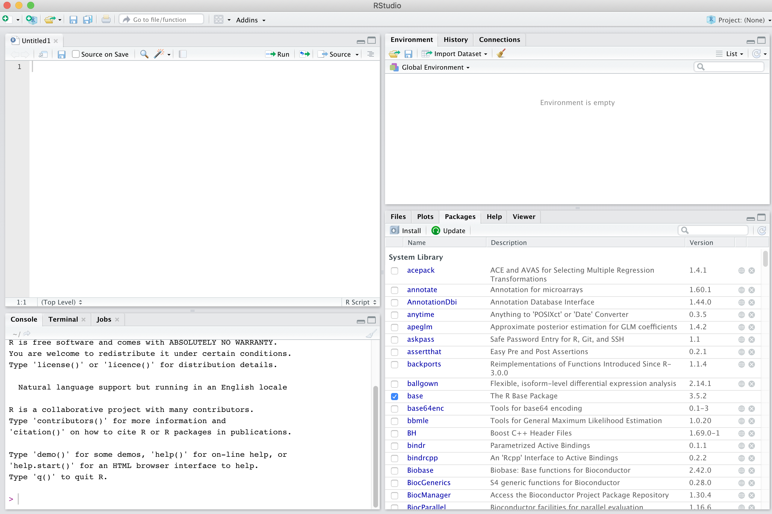
Much of the work you will do will do will happen in the two left panes of R-Studio. These are

• SOURCE which is where you will write your R commands before executing them and

• CONSOLE where the execution happens. The console is the same thing as running R in terminal.

You can always type commands directly in the console without writing them in the source first. This allows you to test commands out. When your workflow begins to get more complex, the source comes in handy.

You will get the hang of R-Studio once we start working through it. The author will explain more features as they become relevant for the task at hand.

3. Getting Started

We will start with very simple tasks and build on that so that by the end of the day you will have a better idea of what R is capable of.

3.1 R as Calculator

At a very basic level, R can be used as a calculator, both simple and scientific. When performing calculations, basic rules of Maths apply i.e. PEMDAS

• Products before Exponents
• Then Exponents
• Multiply and divide before you add or substract

Let’s try some exercises:

489 * 20

5222/40.78

(32*8) + (1000/5.2)

log(7)

log10(7)

550^2

sqrt(302500)

Here are the outcomes:

489 * 20
[1] 9780

5222/40.78
[1] 128.053

(32*8) + (1000/5.2)
[1] 448.3077

log(7)
[1] 1.94591

log10(7)
[1] 0.845098

550^2
[1] 302500

sqrt(302500)
[1] 550

• Try out any other combinations you would like.

3.2 Assignment Operators

Much of the work in this environment is done by manipulating objects that are stored in R’s memory. These objects could be something that was created within R or bringing existing data into the environment. In either case, you will need to make use of the assignment operator <- or =. Both are interchangeable. By far in my experience, most people use the first symbol, though nothing says you have to use one of the other. They are fully equivalent.

• Let’s begin by creating some objects in R through simple assignments:

a <- 8

• This stores the number 8 into an object a. Here is another example:

b <- 22

• You can check for any objects that now exist in R’s memory with the following:

ls()

[1] "a" "b"

• As you can see, both objects are now in R’s memory along with their values.

• Note: ls is a command for listing objects in the working space. The () you see after that is part of R syntax. Every command in R must end with the paranthesis. Although it’s not being implemented here, usually one passes various arguments or options to the command inside those parentheses.

• To check their values, simply type their name at their prompt:

a
[1] 8

b
[1] 22

3.3 Types of Objects

There are many different types of objects that you can store in R’s memory. They can range from very simple numeric objects such as the ones in the examples above, to very complex. The objects can be either singular storing a single number (numeric, or character) or vectors (multiple numbers and/or characters) or large matrices consisting of multiple rows and columns. A typical spreadsheet that we have all worked with in the past is an example of this class of object. Let’s take a look at some moderately complex examples:

• Create a numeric vector and store it in an object:

months <- c(1, 2, 3, 4, 5, 6, 7, 8, 9, 10, 11, 12)

months

 [1]  1  2  3  4  5  6  7  8  9 10 11 12

• Note how the c() or concatenate allows you to create a vector of numbers.

• You could have created this exact same vector another way e.g.

months2 <- 1:12

months2

 [1]  1  2  3  4  5  6  7  8  9 10 11 12

• As you can see, there are multiple methods for performing same operations. The second one took less effort and is smarter. It also omits the usage of the concatenate function.

• Let’s make a character vector

monthsC <- c("January", "February", "March", "April", "May", "June", 
        "July", "August", "September", "October", "November", "December")

monthsC

 [1] "January"   "February"  "March"     "April"     "May"       "June"     
 [7] "July"      "August"    "September" "October"   "November"  "December" 

• What is different about this vector? Notice how unlike the numeric vector, the individual elements in a character vector must be protected by quotes. Try making the same vector without the quotes and see if it works. If not, what error did you get?

3.4 Manipulating Vectors

We can perform various functions on the vectors. For example, if the vectors are of equal length, we can combine them together into a data frame.

year <- data.frame(months, monthsC)

year

   months   monthsC
1       1   January
2       2  February
3       3     March
4       4     April
5       5       May
6       6      June
7       7      July
8       8    August
9       9 September
10     10   October
11     11  November
12     12  December

You will notice that R nicely formats the objects when printing them to the screen. This is quite useful when you are looking at larger data frames.

3.4.1 Task:

• Create a numeric vector (called numdays) containing number of days in each month (assume leap-year) and create a new data frame containing months, monthsC and numdays vectors.

3.5 Creating Data Frames

In our last example, we created a data frame that is a combination of character and numeric vector. But data frames can also be completely numeric, as in the following example:

• Let’s consider an average of monthly high and low tempeartures in Jackson, Wyoming in degrees Celsius.

jackhighC <- c(-2, 0, 6, 11, 17, 23, 28, 27, 22, 14, 4, -2)

jacklowC <- c(-15, -13, -8, -4, 0, 3, 5, 4, 0, -4, -9, -14)

```r


- Now let's make a numeric data frame with these data:


```r

jacktemp <- data.frame(jackhighC, jacklowC)

jacktemp

   jackhighC jacklowC
1         -2      -15
2          0      -13
3          6       -8
4         11       -4
5         17        0
6         23        3
7         28        5
8         27        4
9         22        0
10        14       -4
11         4       -9
12        -2      -14

• Recall that in one of the examples above, we had created a vector of months of the year. Let’s combine that with this data frame.

jacktemp <- data.frame(year, jacktemp)


jacktemp

   months   monthsC jackhighC jacklowC
1       1   January        -2      -15
2       2  February         0      -13
3       3     March         6       -8
4       4     April        11       -4
5       5       May        17        0
6       6      June        23        3
7       7      July        28        5
8       8    August        27        4
9       9 September        22        0
10     10   October        14       -4
11     11  November         4       -9
12     12  December        -2      -14

• Notice that in above example, we overwrote the original data frame jacktemp by concatenating it with the year data frame. But we retained the original name. We could have stored this new data frame under a new name, but the method we used reduces clutter.

• Now let’s convert the temperatures listed in degrees Celsius to degress Fahrenheit. To do this, multiply the tempearature in degC by 9/5, then add the resulting number to 32. For example, if you were converting 4C to Fahrenheight, you would do this:

(4*9/5)+13

• In case of our data frame, we can create and add a new column on the fly to the existing data frame.

jacktemp$jackhighF <- (jacktemp$jackhighC * 9/5) + 32

jacktemp


   months   monthsC jackhighC jacklowC jackhighF
1       1   January        -2      -15      28.4
2       2  February         0      -13      32.0
3       3     March         6       -8      42.8
4       4     April        11       -4      51.8
5       5       May        17        0      62.6
6       6      June        23        3      73.4
7       7      July        28        5      82.4
8       8    August        27        4      80.6
9       9 September        22        0      71.6
10     10   October        14       -4      57.2
11     11  November         4       -9      39.2
12     12  December        -2      -14      28.4

3.5.1 Task:

• Repeat the same process for converting the values from jacklowC column.

3.6 Importing and Working with Data Frames

So far we saw some of the way to generate data within R. But of course, importing data is an integral part of R functionality. We will look at some simple examples first. R provides functions for reading delimited flat text files i.e. .csv (comma separated) and .txt (tab separated).

• We will read estimated U.S. census numbers from year 2018. In your current folder, you will see a file named census.csv. The .csv extension indicates that this is a comma separated file. So we will employ the R function for reading such files.

census <- read.csv("census.csv", header=T)

• Notice the use of assignment operator i.e. <- to send information obtained from read.csv and then storing it inside the object called census. This object name is completely arbitrary. You could use any name you wish, so long as the name is not the same as one of the R functions and the other stipulation is that it may not begin with a number.

• A quick method for checking what the data in an object looks like is to run the head() function on it. For example,

head(census)

       GEO_ID    Location Estimate MarginError
1 0400000US27   Minnesota  5527358       *****
2 0400000US28 Mississippi  2988762       *****
3 0400000US29    Missouri  6090062       *****
4 0400000US30     Montana  1041732       *****
5 0400000US31    Nebraska  1904760       *****
6 0400000US32      Nevada  2922849       *****

This function will always display the first six rows of the data set. Similarly you can check the last six rows with the tail() function.

tail(census)

        GEO_ID      Location  Estimate MarginError
48 0400000US22     Louisiana   4663616       *****
49 0400000US23         Maine   1332813       *****
50 0400000US24      Maryland   6003435       *****
51 0400000US25 Massachusetts   6830193       *****
52 0400000US26      Michigan   9957488       *****
53   0100000US United States 322903030       *****

• Notice how R always formats the data nicely such that the columns are perfectly aligned. It also always shows the header line, even when you are looking at the bottom of the file only.

• You might want to check the dimensions of this data frame (i.e. number of columns and rows).

dim(census)

[1] 53  4

• The first number is for rows and second for columns. There are 53 rows because in addition to the 50 states, we have data on District of Columbia, Puerto Rico and the entire United States.

• If you wanted to check data in other columns and rows that are between those shown by head() and tail() functions, R provides multiple ways to do so. R provides a coordinate system as follows:

  • obj[ROW,COL]

  • For example, to extract row 20 and columns 1:4, you would type this:

  • census[20,1:4]

  • In fact, when asking for all columns in a given row, the column call is superfluous. Instead try this:

  • census[20,] which will provide the exact same information as above.

  
          GEO_ID  Location Estimate MarginError
      20 0400000US47 Tennessee  6651089       *****

  • To get rows from 15 through 25, try census[15:25,]

  
          GEO_ID       Location Estimate MarginError
      15 0400000US41         Oregon  4081943       *****
      16 0400000US42   Pennsylvania 12791181       *****
      17 0400000US44   Rhode Island  1056611       *****
      18 0400000US45 South Carolina  4955925       *****
      19 0400000US46   South Dakota   864289       *****
      20 0400000US47      Tennessee  6651089       *****
      21 0400000US48          Texas 27885195       *****
      22 0400000US49           Utah  3045350       *****
      23 0400000US50        Vermont   624977       *****
      24 0400000US51       Virginia  8413774       *****
      25 0400000US54  West Virginia  1829054       *****

• There is a single column of numeric data in this data frame. What are some of the questions you can ask of this data? Here are a few I came up with:

  1. What is the average state/territory population?
  2. Which states/territories have the largest and smallest populations?

• We can easily answer these questions using functions in R. However, our data set currently has a row containing combined numbers for all states and territories. We can either remove that row entirely, or better yet, make a copy of this data frame without the last row. Here is how to do it:

census2 <- census[1:52,]

• In the above example we are assigning the first 52 rows (header row is automatically copied) of the original data frame to the new frame we are creating on the fly. Check to make sure things look as you expect.

dim(census2)

[1] 52  4

• You can also check the names of states/territories quickly to verify that USA has been excluded:

census2$Location

 [1] Minnesota            Mississippi          Missouri            
 [4] Montana              Nebraska             Nevada              
 [7] New Hampshire        New Jersey           New Mexico          
[10] New York             North Carolina       North Dakota        
[13] Ohio                 Oklahoma             Oregon              
[16] Pennsylvania         Rhode Island         South Carolina      
[19] South Dakota         Tennessee            Texas               
[22] Utah                 Vermont              Virginia            
[25] West Virginia        Washington           Wisconsin           
[28] Wyoming              Puerto Rico          Alabama             
[31] Alaska               Arizona              Arkansas            
[34] California           Colorado             Connecticut         
[37] Delaware             District of Columbia Florida             
[40] Georgia              Idaho                Hawaii              
[43] Illinois             Indiana              Iowa                
[46] Kansas               Kentucky             Louisiana           
[49] Maine                Maryland             Massachusetts       
[52] Michigan            

• All looks good here. Now let’s get the answers to our questions:

min(census2$Estimate)

[1] 581836

• Now we know the lowest population size, but we don’t know what state that belongs to. We can find that out with the subset function:

subset(census2, Estimate == 581836)

        GEO_ID Location Estimate MarginError
28 0400000US56  Wyoming   581836       *****

• No surprises there!

3.6.1 Task:

• Find out which state has the largest population.

4. Maintaining Your R Installation

There are a few housekeeping tasks you will need to do maintain your R installation on a regular basis. This involves keeping your base-R version, R-Studio installation as well as various additional packages updated. Installing a new version of R often breaks existing packages, which would then have to be updated as well. Updating the R installation is as simple as going to r-project.org and downloading/installing the latest version. Unfortunately given the administrative permissions on the workstations you are working on right now, we can’t really try this out. However, we will tackle the subject of packages next.

4.1 What is an R Package?

Some of you might be wondering what an R package is? It’s a fair question that baffles many beginner R users. Remember that we talked earlier about base-R distribution, which includes a core set of functions to work with data. We visited some of these functions above. But R is now used in a large number of disparate scientific fields scattered across industry, academic, government and non-government entities. This means need for highly specialized functions to do specific tasks that are not included in your base-R distribution.

A R package is simply a collection of functions that perform specialized tasks. Data scientists and enthusiasts alike volunteer their valuable time to develop such specialized packages and then make them avaialble to the larger user base free of charge.

We can think of an analogy here. Your smartphone operating system comes with a suite of basic functions that allow your to make and receive phone calls and text messages. However, if you need to do a video chat, you will need a special app for that. To check your email, you will need another app. An app here is highly similar to a package capable of doing specific tasks.

There are literally thousands of R packages available. To give you a few example:

• ggplot2 is used extensively in data visualization
• vegan is a package that contains a larger number of statistical tests
• RMarkdown allows generation of dynamic documents such as the one you are currently reading
• Parallel splits data analysis jobs into chunks so they can be completed faster by multiple processors

So on and so forth.

4.2 Package Repositories

You can download and install packages from several sources, though of course not all packages are avaialble from all sources. These sources are also called as repositories. There are three main repositories that you should be aware of:

• CRAN: The Comprehensive R Archive Network located at CRAN.r-project.org: This is by far the biggest and most vetted repository of packages that are available. Before a package appears in the CRAN repository, it must be submitted for review and thoroughly vetted and approved by the folks responsible for CRAN. As of today, there are 15,364 packages available there.

• Bioconductor: Is the repository to go to if you are looking for biological analysis software e.g. bioinformatics packages. This repository is located at bioconductor.org and currently contains 1,823 packages.

• GitHub: has become the de-facto place to share cutting edge developments for many of the packages available on the above two repositories. Often times when package installation fails due to incompatibility between the R version and the package, you can find the source code for the package on this repository and circumvent the compatibility problems associated with pre-compiled packages. It’s too difficult to count the number of package sources available on GitHub. But it will be easy to find what you need when you need it.

4.3 Installing and Loading Packages

There are several ways of installing R packages:

• Most package from CRAN can be installed with the function install.packages(). For example, let’s try installing one:

install.packages("vegan")

When you launch this command for the first time, a dialogue box will pop out on your screen asking you to choose a mirror for installation. What is a mirror you might ask? Because R packages are installed from all over the world, repositories make their packages available on a number of web servers (called a mirror here) around the world. The idea is that by choosing a mirror closest to you, the download speeds would be the highest you can get.

If the above command was successful, the package was installed. However, that doesn’t automatically make the package functions available for your use. You must first load the package in R’s memory. Here is how to do it:

load(vegan)

Note how we used quotes around the package name when installing it but not when loading it. If you deviate from this convention, R will generate an error message.

• Bioconductor packages require special commands for installation. Let’s try installing the package DESeq2. If you go the package webpage, you will find an installation section. It consists of two separate commands:

if (!requireNamespace("BiocManager", quietly = TRUE))
    install.packages("BiocManager")

This loads the script called BiocManager on your computer, which is needed for installation of every bioconductor package. Next, install the package:

BiocManager::install("DESeq2")

• There are two circumstances under which you will need to access package source code on GitHub. One scenario is that your R version is incompatible with the package you are trying to install from CRAN. Alternatively, you may find that the package version on CRAN is outdated and you want access to new functionality included only in the source code available on GitHub. In either of these cases, here is how to install an R package from source:

• First, you will need a package called devtools

library(devtools)

• If the above command fails, you will need to install devtools first. But assuming this worked, let’s install a package called RMarkdown.

library(devtools)

devtools::install_github("rstudio/rmarkdown")

• In the above example, the rstudio part is the name of the author/account on GitHub and rmarkdown is the name of the package.

4.3.1 Task:

Install the tidyverse family of packages from GitHub. Their address is: github.com/hadley/tidyverse.

4.4 Getting Help Within R

R-Studio provides a nice interface for accessing help documentation within R, but you can also search for help through the console window. Invoking help pages for any function is done by simply typing the name of the function preceded by a question mark. Try the following out.

?plot

?mean

?sum

?hist

?cor.test

4.5 Getting Help from Fellow R Users

R has become extremely popular as a powerful statistical analysis program in all sectors e.g. academics, industry, government and NGOs. Consequently, there are a number of websites, forums and mailing lists that are available to you. When you run into a problem with your code and any R function, chances are that someone has already asked a question about it which has been answered. Below is a list of resources that you might find helpful.

• R-Help Mailing List

• Topic Specific Mailing Lists

• StackOverFlow.com

• R-Studio Community

• Bioconductor Support Forum

• Freenode ##r Channel on IRC

5. Statistical Analysis

R provides numerous functions for performing statistical analysis on a wide variety of data sets. In this section, We will both import example data and also create some on the fly within R.

5.1 Summarizing Data

Here we will look at some of the most commonly used summarizing statistics:

• Sum
• Mean / Average
• Median
• Largest value
• Smallest value
• Standard Deviation
• Variance
• Number of Elements

• Let’s bring in a commonly used data set that is built into R: mtcars

data(mtcars)

• Quickly look at the help pages for this data set

?mtcars

mtcars                package:datasets                 R Documentation

Motor Trend Car Road Tests

Description:

     The data was extracted from the 1974 _Motor Trend_ US magazine,
     and comprises fuel consumption and 10 aspects of automobile design
     and performance for 32 automobiles (1973-74 models).

Usage:

     mtcars
     
Format:

     A data frame with 32 observations on 11 (numeric) variables.

       [, 1]  mpg   Miles/(US) gallon                        
       [, 2]  cyl   Number of cylinders                      
       [, 3]  disp  Displacement (cu.in.)                    
       [, 4]  hp    Gross horsepower                         
       [, 5]  drat  Rear axle ratio                          
       [, 6]  wt    Weight (1000 lbs)                        
       [, 7]  qsec  1/4 mile time                            
       [, 8]  vs    Engine (0 = V-shaped, 1 = straight)      
       [, 9]  am    Transmission (0 = automatic, 1 = manual) 
       [,10]  gear  Number of forward gears                  
       [,11]  carb  Number of carburetors                 

• Let’s say we want to find out the car make with lowest and highest gas mileage:

min(mtcars$mpg)

[1] 10.4
 
subset(mtcars, mpg == 10.4)

                     mpg cyl disp  hp drat    wt  qsec vs am gear carb
Cadillac Fleetwood  10.4   8  472 205 2.93 5.250 17.98  0  0    3    4
Lincoln Continental 10.4   8  460 215 3.00 5.424 17.82  0  0    3    4

• Thus there are two cars with lowest gas mileage. Now check for high.

subset(mtcars, mpg == 33.9)

                mpg cyl disp hp drat    wt qsec vs am gear carb
Toyota Corolla 33.9   4 71.1 65 4.22 1.835 19.9  1  1    4    1

• What is the average gas mileage across all vehicles?

mean(mtcars$mpg)

[1] 20.09062

• Note that this is not a discrete number so you couldn’t subset the dataset using it to find the car with average gas mileage. Instead you can apply a conditional:

subset(mtcars, mpg < 21 & mpg > 19)

                  mpg cyl  disp  hp drat    wt  qsec vs am gear carb
Merc 280         19.2   6 167.6 123 3.92 3.440 18.30  1  0    4    4
Pontiac Firebird 19.2   8 400.0 175 3.08 3.845 17.05  0  0    3    2
Ferrari Dino     19.7   6 145.0 175 3.62 2.770 15.50  0  1    5    6

• What about variance and standard deviation in gas mileage?

var(mtcars$mpg)
[1] 36.3241
 
sd(mtcars$mpg)
[1] 6.026948

• Finally, you can also get all summary statistics for each variable included in this data set with just one function:

summary(mtcars)

      mpg             cyl             disp             hp       
 Min.   :10.40   Min.   :4.000   Min.   : 71.1   Min.   : 52.0  
 1st Qu.:15.43   1st Qu.:4.000   1st Qu.:120.8   1st Qu.: 96.5  
 Median :19.20   Median :6.000   Median :196.3   Median :123.0  
 Mean   :20.09   Mean   :6.188   Mean   :230.7   Mean   :146.7  
 3rd Qu.:22.80   3rd Qu.:8.000   3rd Qu.:326.0   3rd Qu.:180.0  
 Max.   :33.90   Max.   :8.000   Max.   :472.0   Max.   :335.0  
      drat             wt             qsec             vs        
 Min.   :2.760   Min.   :1.513   Min.   :14.50   Min.   :0.0000  
 1st Qu.:3.080   1st Qu.:2.581   1st Qu.:16.89   1st Qu.:0.0000  
 Median :3.695   Median :3.325   Median :17.71   Median :0.0000  
 Mean   :3.597   Mean   :3.217   Mean   :17.85   Mean   :0.4375  
 3rd Qu.:3.920   3rd Qu.:3.610   3rd Qu.:18.90   3rd Qu.:1.0000  
 Max.   :4.930   Max.   :5.424   Max.   :22.90   Max.   :1.0000  
       am              gear            carb      
 Min.   :0.0000   Min.   :3.000   Min.   :1.000  
 1st Qu.:0.0000   1st Qu.:3.000   1st Qu.:2.000  
 Median :0.0000   Median :4.000   Median :2.000  
 Mean   :0.4062   Mean   :3.688   Mean   :2.812  
 3rd Qu.:1.0000   3rd Qu.:4.000   3rd Qu.:4.000  
 Max.   :1.0000   Max.   :5.000   Max.   :8.000  

5.1.1 Task:

• Load the data on approval ratings of U.S. presidents since 1945 through 1975. The dataset is named presidents.

• Examine the data structure (hint: head, tail etc.)

• Analyze a summary of each variable in the data set

5.2 Simulating Distributions

• Imagine you wish to create a vector of normally distributed numbers with stated mean and standard deviation. Then you want to test how well the vector conforms to the bell shaped curve you envision for normal distribution.

rnorm(10, 0, 1)

 [1] -0.07464322 -1.51165519  0.24215035 -1.01457525  0.12778428 -0.39497391
 [7] -1.98659094 -0.01535476 -1.90261294  0.76944419

• Here we are using the function rnorm() which takes three arguments:

  • rnorm(length, mean, sd)
  • length = Number of values in the vector
  • mean = mean value of the entire distribution
  • sd = standard deviation around the mean

• In the above example, we asked for length=10, mean=0 and sd=1.

• Let’s create 4 additional vectors of variable length all with a mean of 5 and standard deviation of 2.

norm10 <- rnorm(10, 5, 2)

norm100 <- rnorm(100, 5, 2)

norm1k <- rnorm(1000, 5, 2)

norm100k <- rnorm(100000, 5, 2)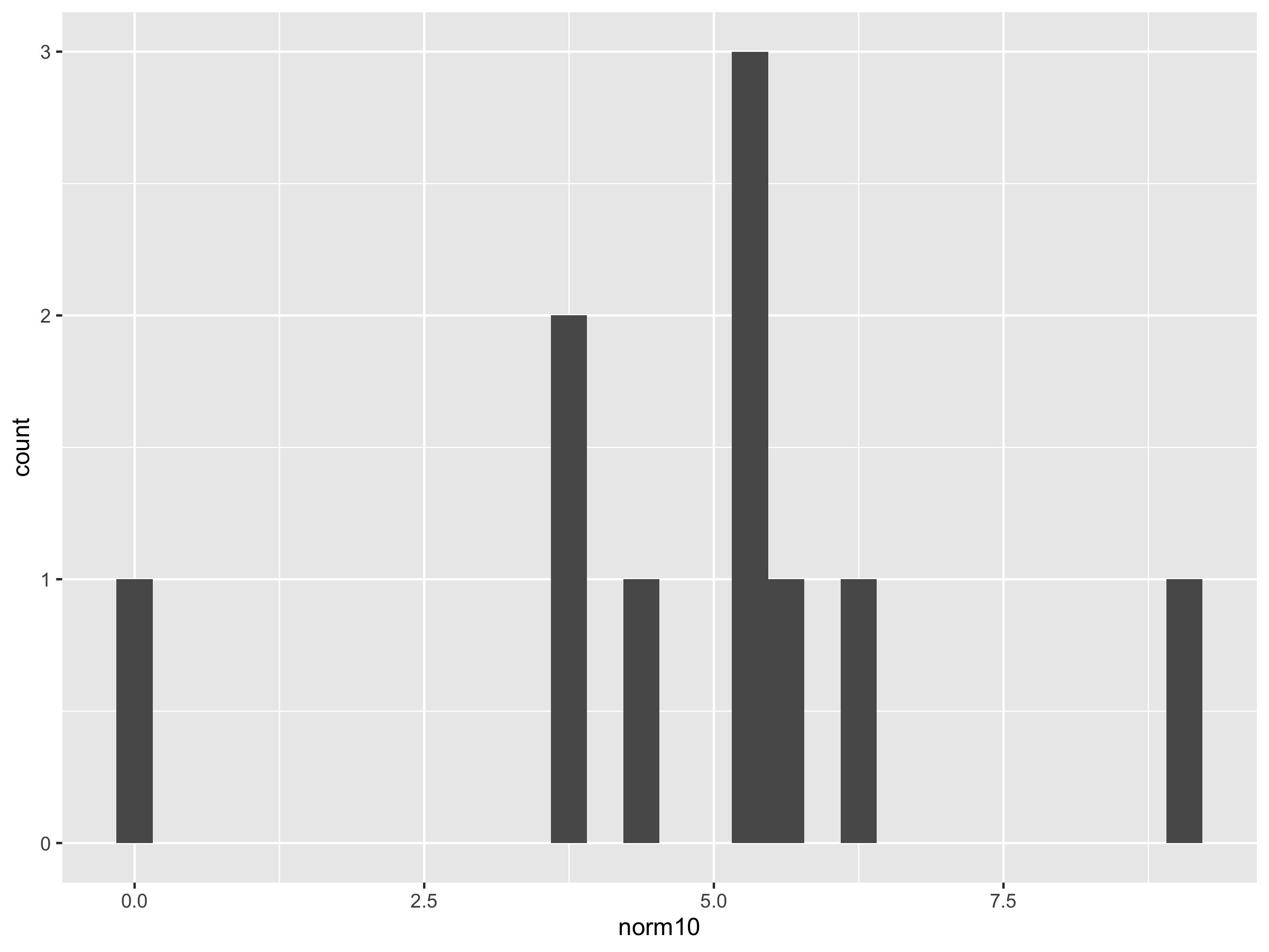

• Now let’s visualize how well these distributions conform to the bell shape characteristic of the normal distribution.

library(tidyverse)

ggplot() + geom_histogram(aes(norm10))

• This looks rather crude. Go on and create the remaining three histograms using the same method and observe how they differ from each other.

ggplot() + geom_histogram(aes(norm100))

ggplot() + geom_histogram(aes(norm1k))

ggplot() + geom_histogram(aes(norm100k))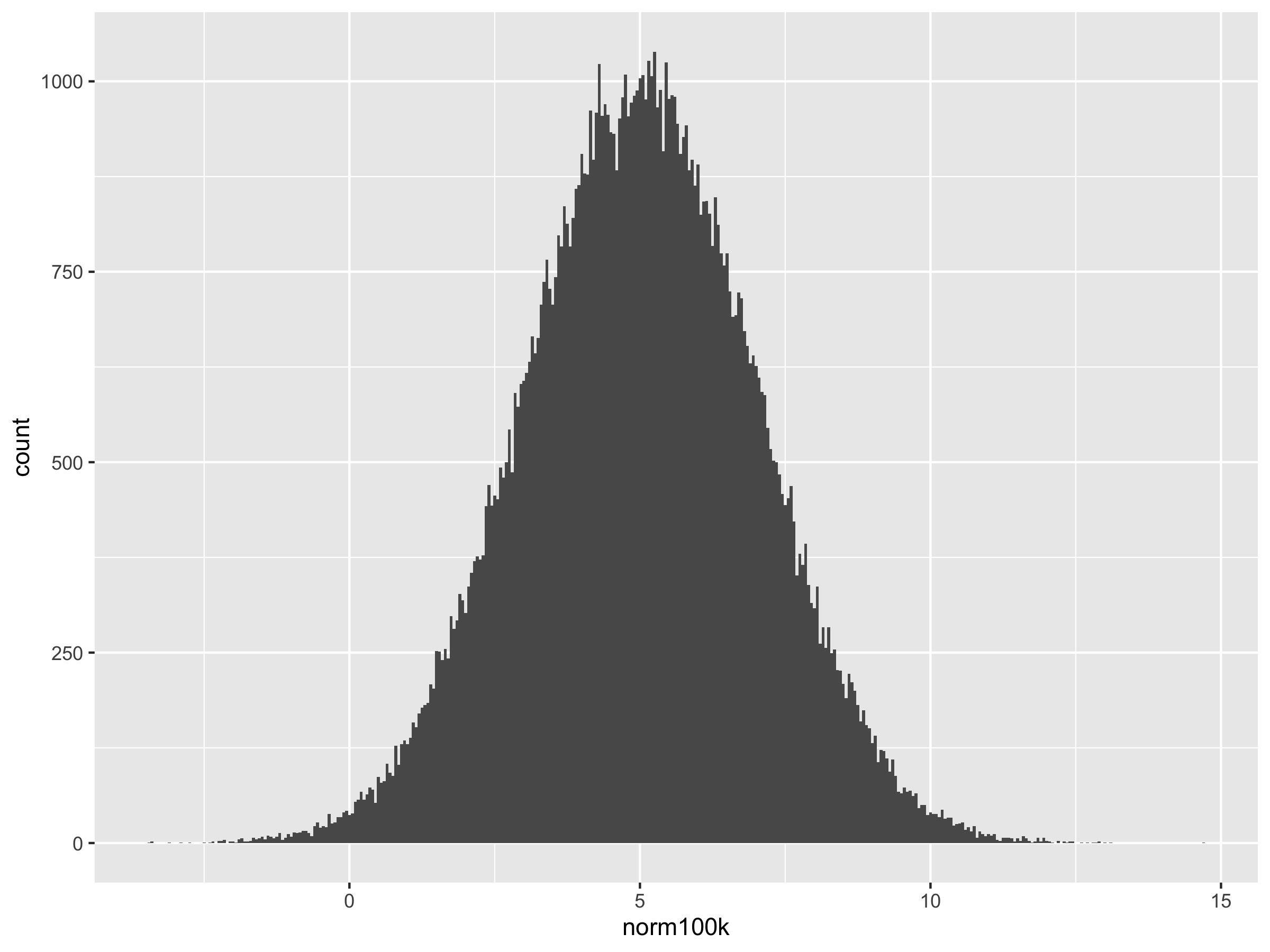

• This suggests that larger vectors will show a better conformance to the bell curve than smaller ones.

5.2.1 Task:

• The R function which deals with Uniform Distribution is named runif. Look at the help page for it.

• Simulate two vectors, one of length 100 and another of 1 million and store them in different objects.

• Draw a histogram of each vector to examine the shape of the distribution and identify any differences.

5.3 Sampling

It is possible to randomly sample data from a distribution. The sample() function takes two arguments.

• sample(vector, n, replace=VALUE)

• Where vector = distribution, n = size of your sample

sample(1:25, 5, replace=TRUE)

[1]  3 13  4  6  7

• The argument replace can be set to either TRUE or FALSE depending upon whether your experiment allows re-sampling of the same value across successive iterations. However, it must be set to TRUE if your sample size exceeds the size of the vector. In other words, if you are sampling a vector of length 10, fifteen times, you will run out of numbers if replace was set to FALSE. Try the following example:

sample(1:10, 15, replace=FALSE)

Error in sample.int(length(x), size, replace, prob) : 
  cannot take a sample larger than the population when 'replace = FALSE'


sample(1:10, 15, replace=TRUE)

 [1]  7  3 10  4  5  3  5  7 10  3 10  1  2  4  2

• Also notice how the sample changes every time you repeat the exact same command. This is because the sample is randomized by default.

sample(1:10, 15, replace=TRUE)

 [1] 6 8 8 6 3 9 7 2 6 5 1 6 5 3 2

• Of course, sometimes you need to be able to replicate your results precisely. In those instances, you can set the seed as follows:

sed.seed(5)

sample(500:1000, 50, replace=TRUE)

 [1] 821 862 684 706 702 876 796 712 721 570 902 886 793 813 930 808 831 515 909
[20] 984 627 526 956 969 719 829 584 621 973 806 612 937 683 591 768 962 906 734
[39] 553 929 645 963 691 652 893 797 615 747 507 967

• Seed can be set to any number you wish. Using the same seed again will reproduce your original sample. Try running the command again with the same seed to verify.

• Now draw the sample again without setting the seed and you will notice that it changes again.

sample(500:1000, 50, replace=TRUE)

 [1] 719 903 864 990 603 735 944 622 962 825 648 590 854 571 550 933 579 919 507
[20] 980 965 831 815 880 589 626 724 514 873 599 708 647 624 741 638 636 503 502
[39] 911 654 726 503 526 739 668 921 629 771 904 687

• The set.seed() function is extremely useful for achieving reproducibility. You may use it with any function in R, not just sample.

• Sample function works both with numerical and character data. Let’s consider an example from genetics. Imagine you wish to create a population of 200 individuals to to study a gene A. This gene appears in the population in 2 forms: A and a. Because all the individuals have two sets of genes (hence called diploid), there are three distinct possibilities for the genetic makeup of each individual:

• AA or Aa or aa

pop <- sample(c("AA", "Aa", "aa"), 200, replace=TRUE)

pop

  [1] "AA" "AA" "AA" "Aa" "aa" "aa" "AA" "Aa" "AA" "AA" "Aa" "aa" "Aa" "AA" "aa"
 [16] "Aa" "AA" "aa" "aa" "Aa" "Aa" "Aa" "Aa" "aa" "aa" "aa" "AA" "aa" "AA" "aa"
 [31] "Aa" "aa" "aa" "AA" "AA" "Aa" "Aa" "AA" "Aa" "AA" "AA" "Aa" "aa" "AA" "AA"
 [46] "aa" "Aa" "aa" "AA" "Aa" "aa" "aa" "aa" "Aa" "AA" "Aa" "aa" "AA" "AA" "Aa"
 [61] "aa" "aa" "Aa" "AA" "aa" "Aa" "AA" "aa" "aa" "AA" "aa" "AA" "Aa" "AA" "AA"
 [76] "AA" "aa" "Aa" "aa" "aa" "aa" "AA" "AA" "aa" "aa" "AA" "AA" "Aa" "AA" "Aa"
 [91] "aa" "AA" "aa" "aa" "aa" "Aa" "aa" "aa" "aa" "Aa" "AA" "AA" "aa" "aa" "aa"
[106] "Aa" "AA" "AA" "Aa" "Aa" "aa" "Aa" "Aa" "aa" "AA" "aa" "aa" "aa" "AA" "aa"
[121] "AA" "Aa" "AA" "AA" "AA" "Aa" "aa" "AA" "AA" "aa" "aa" "Aa" "AA" "aa" "Aa"
[136] "Aa" "AA" "aa" "Aa" "aa" "aa" "AA" "AA" "Aa" "aa" "Aa" "AA" "Aa" "AA" "AA"
[151] "aa" "AA" "AA" "AA" "Aa" "aa" "AA" "AA" "Aa" "Aa" "aa" "aa" "Aa" "Aa" "Aa"
[166] "AA" "AA" "aa" "aa" "aa" "Aa" "Aa" "AA" "Aa" "Aa" "aa" "aa" "AA" "AA" "AA"
[181] "aa" "AA" "Aa" "AA" "Aa" "Aa" "Aa" "AA" "Aa" "Aa" "aa" "aa" "aa" "aa" "Aa"
[196] "Aa" "AA" "AA" "AA" "aa"

• You could further subsample from this sample to make mini populations and then count the number of individuals of different genetic makeup.

pop1 <- sample(pop, 50, replace=TRUE)

pop1

 [1] "aa" "AA" "AA" "AA" "AA" "Aa" "AA" "aa" "AA" "Aa" "aa" "AA" "aa" "Aa" "Aa"
[16] "Aa" "aa" "aa" "Aa" "Aa" "AA" "aa" "aa" "aa" "aa" "aa" "aa" "AA" "aa" "aa"
[31] "Aa" "Aa" "aa" "AA" "AA" "Aa" "Aa" "Aa" "aa" "aa" "aa" "aa" "Aa" "aa" "aa"
[46] "Aa" "aa" "aa" "AA" "AA"


sum(pop1 == "AA")
[1] 13

sum(pop1 == "Aa")
[1] 14

sum(pop1 == "aa")
[1] 23

• In addition to vectors, R also allows you to sample data frames. Take for example he airquality data set from New York City.

data(airquality)

dim(airquality)
[1] 153   6


head(airquality)

    Ozone Solar.R Wind Temp Month Day
1      41     190  7.4   67     5   1
2      36     118  8.0   72     5   2
3      12     149 12.6   74     5   3
4      18     313 11.5   62     5   4
5      NA      NA 14.3   56     5   5
6      28      NA 14.9   66     5   6

• There are 153 rows in the data set. What if you wanted to take a random sample of 50 rows from this data? Here is the syntax for how to do it:

DATA[sample(nrow(DATA), 50, replace=FALSE), ]

• Just replace the DATA part with the name of our data set.

5.3.1 Task:

• From a character vector containing HEADS and TAILS, randomly take a sample of length 1000.

• Count how many HEADS were sampled.

5.4 Repetitive Tasks

When analyzing any type of data, you may encounter the need for repetition, where a given task needs to be repeated a number of times. If you need to repeat just a handful of times, then you can afford to run it manually. If even 10 repetitions are needed, you would save a lot of time by automating these tasks through loops. A very popular type of loop is called a for() loop. Some programmers will argue that loops are very slow to operate, but this really isn’t a concern when repeating smaller tasks. Let’s look at some examples:

• Print numbers from 1 to 20

for (i in 1:20){
    print(i)
}

[1] 1
[1] 2
[1] 3
[1] 4
[1] 5
[1] 6
[1] 7
[1] 8
[1] 9
[1] 10
[1] 11
[1] 12
[1] 13
[1] 14
[1] 15
[1] 16
[1] 17
[1] 18
[1] 19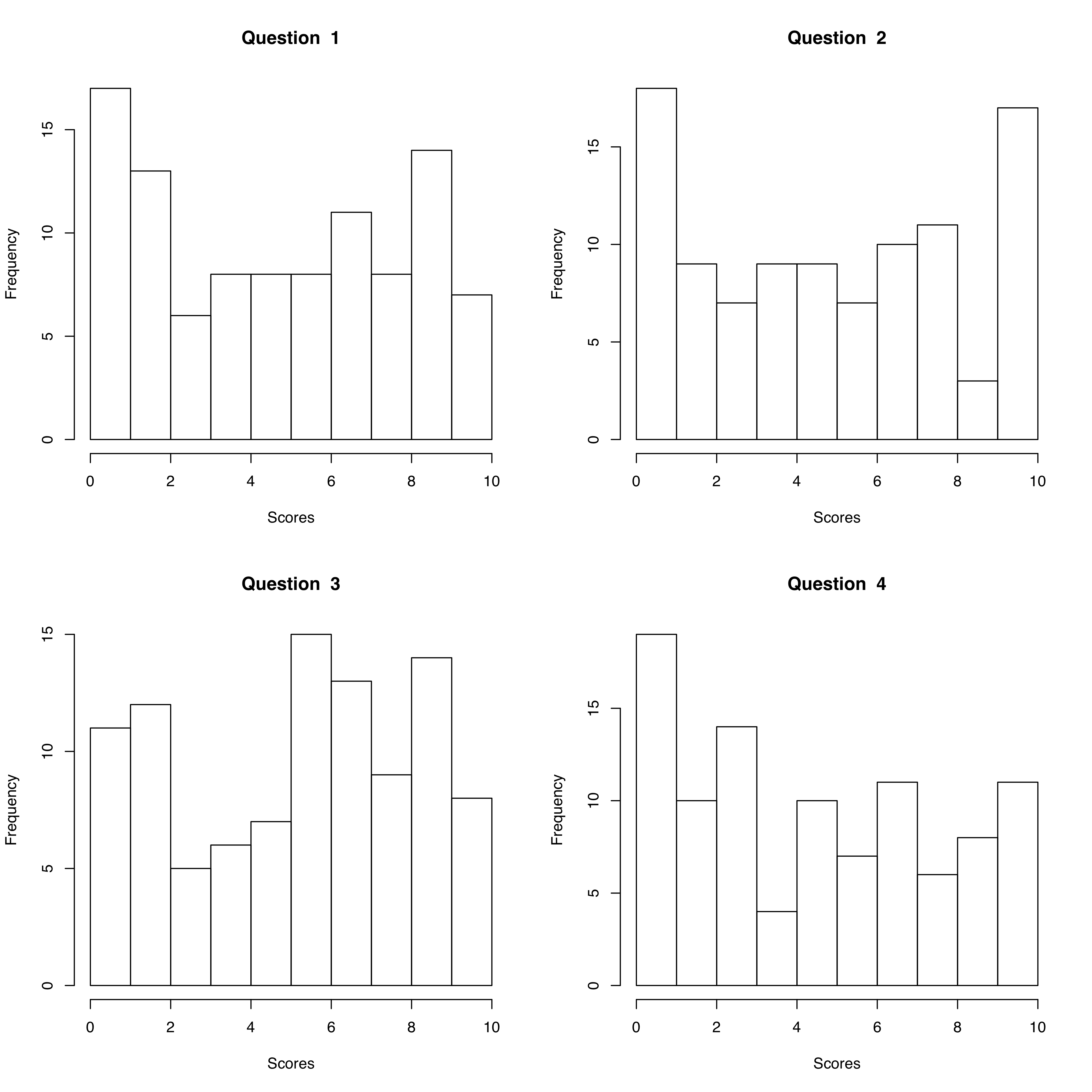
[1] 20

• Print square of a set of numbers

for (i in 1:10){
    print(i^2)
}


[1] 1
[1] 4
[1] 9
[1] 16
[1] 25
[1] 36
[1] 49
[1] 64
[1] 81
[1] 100

• for() loops are also commonly used when generating a number of similar plots from the same data set. Consider a data set where exam scores are recorded for 200 students. Each student has to answer four questions and their grade for each question ranges between 0 and 10. First, let’s creat this data within R using the sample function.

• Generate 100 integers between 0 and 10 with replacement.

sample(0:10, 100, replace=TRUE)

  [1] 10  6  3  2  5  3 10 10  1  2 10  9  8 10  7  3  8  1  4  9 10  4  3  3  6
 [26] 10  8  2  9  7  1 10  0  4  0  3 10  5  6  2  8  8  5  4  8  9  5 10  5  7
 [51]  6  5  9  9  0 10 10  9  7  5  0  0  6  4  5  9  2 10  9  1  5  2  2  7 10
 [76]  7  6  4  3  7  6  5  2 10 10  4  4  9  0  2  8  1  1  5  0  3  3  8  2  5

• These are randomly generated numbers and would become scores for 100 people for one of the questions. Now we just need to repeat this process 4 times.

replicate(4, sample(0:10, 100, replace=TRUE))

       [,1] [,2] [,3] [,4]
  [1,]    8    4    1    0
  [2,]    7    2    8   10
  [3,]    1    5    5    1
  [4,]   10    7    7    1
  [5,]    8    1    0    0
  [6,]    0    2    4    5
  [7,]    6    9   10    9
  [8,]    9    4    9    6
  [9,]    2    0   10    5
 [10,]    9    0    5    9
 [11,]    5    7    2    9
 [12,]    9    6    7    2
 [13,]    8    9    7    3
 [14,]    3   10    8    0
 [15,]    0    3    4   10
 [16,]    9    7    4    8
 [17,]    7    9    1    3
 [18,]    3    6   10    1
 [19,]    3    0    7    5
 [20,]    5    5   10   10
 [21,]    3   10    8    1
 [22,]    6    0   10    5
 [23,]    4    1    4    8
 [24,]    7    1    4   10
 [25,]    5    8    1    6
 [26,]   10    3    2    9
 [27,]    7    8    0    8
 [28,]    2    4    2    5
 [29,]    4    9    7    6
 [30,]    4    5    9    0
 [31,]    3   10    8    2
 [32,]    1    2    8    2
 [33,]    7   10    5    8
 [34,]    5    5    0    7
 [35,]    8    6   10    9
 [36,]    2    0    4    6
 [37,]    1    6    5    7
 [38,]   10    5   10    4
 [39,]    7    3    4    5
 [40,]    9    6    8   10
 [41,]    1    3    1    8
 [42,]    8    4    5    8
 [43,]    1    5    8    7
 [44,]    3    3    0   10
 [45,]    1    4    8    1
 [46,]    4    6    4    5
 [47,]    7   10    8    5
 [48,]    9    3    1    0
 [49,]    3    0    5    2
 [50,]    1    9    9    6
 [51,]    6    5    4    1
 [52,]    4    7    0    9
 [53,]    1    9   10    0
 [54,]    5    3    6    6
 [55,]    9    2    7    8
 [56,]    7   10    7    5
 [57,]    5   10    7   10
 [58,]   10    5    9    6
 [59,]    6    4    1    4
 [60,]    2    2    6   10
 [61,]    3    8    3    5
 [62,]    2    1    4    4
 [63,]   10    1    8    5
 [64,]   10    0    3    2
 [65,]    6    5    0    1
 [66,]    9    4    7    1
 [67,]    6    9    5    5
 [68,]    8    8    9    8
 [69,]    4    8    1    0
 [70,]    4    5    3    0
 [71,]    5    8    0    5
 [72,]    3    3    0   10
 [73,]    0   10    7    3
 [74,]    1    5    0    5
 [75,]    6    6    5    9
 [76,]    2    3    5    7
 [77,]    8    7    9    3
 [78,]    9    5    2   10
 [79,]    0    7    3    6
 [80,]    0    0   10    3
 [81,]    7    3    1   10
 [82,]    9    4   10    6
 [83,]    1    9    7    5
 [84,]    2    8    5    1
 [85,]    3    5   10    8
 [86,]    4    5    0   10
 [87,]    4    9    8    8
 [88,]    2    1    3    9
 [89,]    3    0    2    8
 [90,]    6    8    6    5
 [91,]    4    6    9    0
 [92,]    2    7    2    2
 [93,]    2    0    4   10
 [94,]    2    7    7    8
 [95,]    8    0    9    0
 [96,]    0    1   10    7
 [97,]   10    7    6    2
 [98,]    1    4    3    7
 [99,]    0    2    6    7
[100,]    9    0    2    8

• Now that we know this works, we can save the data into a data frame object.

scores <- replicate(4, sample(0:10, 100, replace=TRUE))

• Check dimensions of the scores

dim(scores)

[1] 100   4

• That’s 100 rows (i.e. 100 students) and 4 scores.

• Now you want to make histograms for each of these four scores to get a visual of how the class performed on the exam overall.

• Before making the loop, first make one histogram:

hist(scores[,1], xlab="Question 1")

• Now we can proceed with setting up the loop.

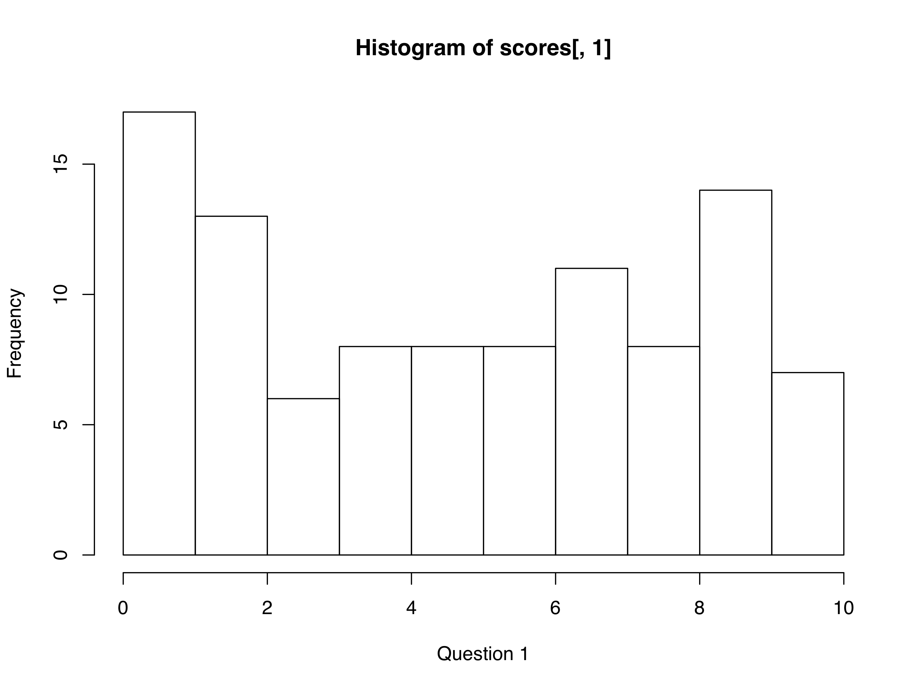
par(mfrow=c(2,2))       

for (i in 1:4){         
    x <- scores[,i]     
    hist(x,
        main = paste("Question ", i),
        xlab = "Scores",
        xlim = c(0,10))
}

5.4.1 Task:

• Load the U.S. states data (data(state)) and check the data frame called state.x77.

• Modify the loop above to plot two histograms from this data frame, one each for population and Area.

5.5 Student’s T-test

Also called just the T-test is used to compare mean values of two samples that are assumed to be normally distributed. T-test is a parametric test. The goal is to test whether means of two samples are significantly different from each other.

• First we need two normally distributed samples

x <- rnorm(1000)

y <- rnorm(1000)

t.test(x, y)

    Welch Two Sample t-test

data:  x and y
t = 1.0993, df = 1998, p-value = 0.2718
alternative hypothesis: true difference in means is not equal to 0
95 percent confidence interval:
 -0.03860205  0.13706775
sample estimates:
  mean of x   mean of y 
-0.02702567 -0.07625852 

• This result shows that the means of the two samples x and y are not significantly different from each other (P-value 0.2718).
• Let’s arbitrarily set the two samples with different means and recheck

a <- rnorm(1000, mean=2)

b <- rnorm(1000, mean=4)

t.test(a, b)

    Welch Two Sample t-test

data:  a and b
t = -44.009, df = 1997.8, p-value < 2.2e-16
alternative hypothesis: true difference in means is not equal to 0
95 percent confidence interval:
 -2.073730 -1.896795
sample estimates:
mean of x mean of y 
 2.023478  4.008740 

5.5.1 Task:

• Generate two normally distributed vectors, both with a mean of 0.8.

• Compare their with the T-test and observe whether they have similar or different means.

5.6 Chi-Squared Test

This test is done to test how observed values fit to expectations based on principles. In other words it’s a goodness of fit test. Let’s do an example from population genetics. There is a fundamental theorem in population genetics called the Hardy Weinberg Equilibrium. HWE for short provides for expected proportions of genotypes in a population if it conforms to certain assumptions. We do not need to get into these assumption.

• Consider a population of 5000 diploid individuals in which we are studying a gene named F, which has two morphs/alleles/forms: F and f.

• Because the organism is diploid, each individual has two copies of this gene (by way of having two chromosomes of each type.

• Therefore we have three possible types of individual genotypes at this gene: FF, Ff and ff

• HWE posits that genotypic frequencies will add up to unity if the population conforms to certain assumptions.

  • p² + 2pq + q² = 1 where p & q are frequencies of alleles F and f respectively.

• We can use chi square test to check whether our sampled population is in HWE for gene F.

• First, let’s sample a population

pop <- sample(c("FF", "Ff", "ff"), 5000, replace=TRUE)

length(pop)
[1] 5000

• Estimate the number of genotypes of each type

sum(pop == 'FF')
[1] 1726

sum(pop == 'Ff')
[1] 1626

sum(pop == 'ff')
[1] 1648

• Now we can estimate the frequencies of alleles F (p) and f (q) respectively:

p <- (sum(pop == "FF")*2 + sum(pop == "Ff"))/10000

q = (sum(pop == "ff")*2 + sum(pop == "Ff"))/10000

• The allele frequencies of two alleles must always add up to 1. Do they?

p + q 
[1] 1

• We can estimate Expected genotypic frequencies based on allele frequencies

  • freq(FF) = p²
  • freq(Ff) = 2 * p * q
  • freq(ff) = q²

p^2
[1] 0.2578608

q^2
[1] 0.2422608

2*p*q
[1] 0.4998783

• From expected genotypic frequencies we can estimate expected numbers:

0.2578608 * 5000
[1] 1289.304


0.2422608 * 5000
[1] 1211.304


0.4998783 * 5000
[1] 2499.392

• In contrast, our observed numbers for the same genotypes are: 1726, 1648 and 1626.

• Now we can set up the Chi Square Test

• The calculated chi square value is 610, far larger than the value of 5.99 for 2 degrees of freedom (we have three observations). So the population we created is not in Hardy Weinberg Equilibrium. We can reject the null hypothesis.

5.7 Correlation Tests

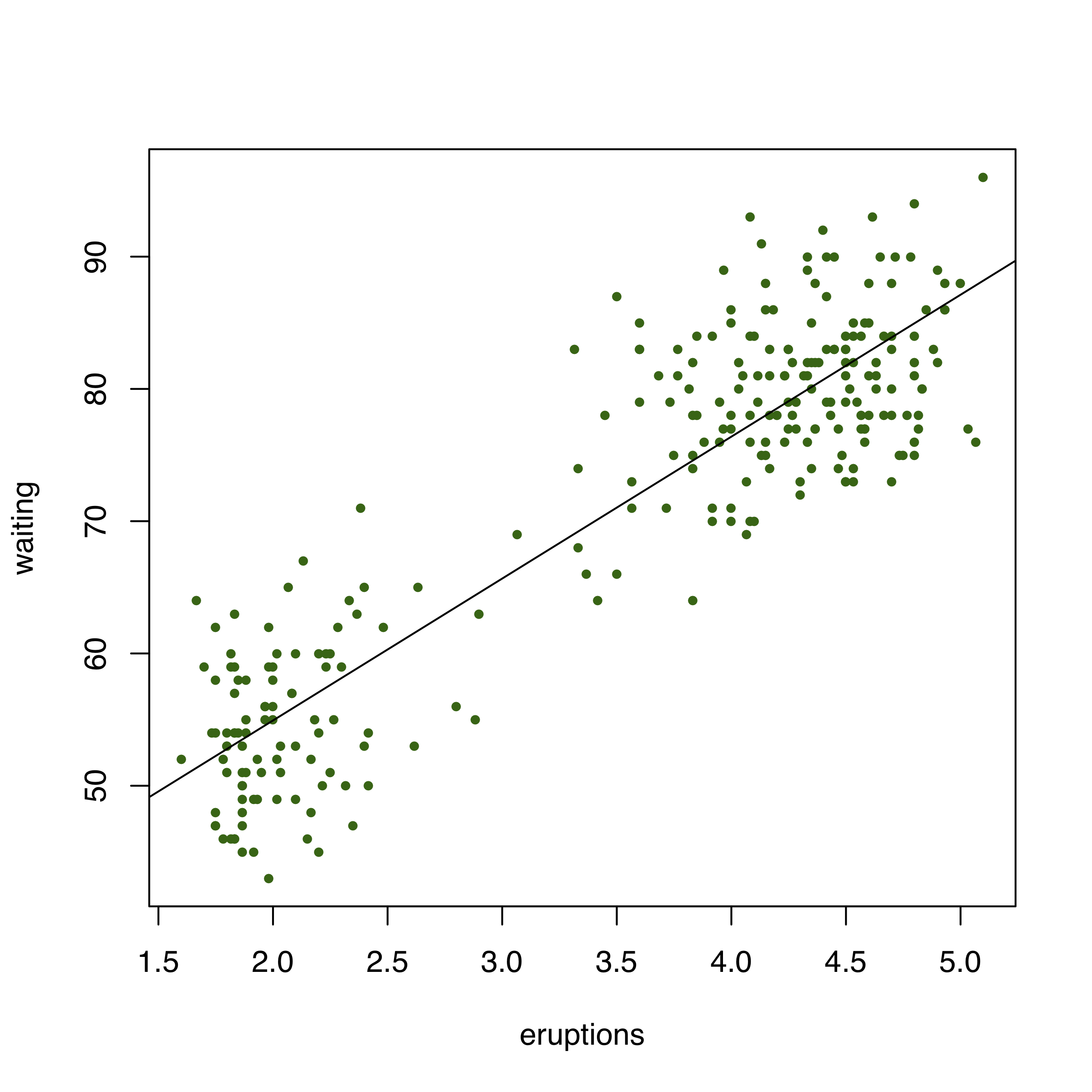
Testing for correlation between two variables is done through multiple functions in R. But not all of them provide significance testing. We will use the function cor.test which provides significance values for the correlation tests and it also allows us to test with different methods e.g. Spearman vs Pearson.

We will use the Faithful dataset built into R, which has eruption duration and wait times between eruptions for the Old Faithful geyser in Yellowstone NP.

• First, load and attach the dataset:

data(faithful)

attach(faithful)

cor.test(eruptions, waiting)

    Pearson's product-moment correlation

data:  eruptions and waiting
t = 34.089, df = 270, p-value < 2.2e-16
alternative hypothesis: true correlation is not equal to 0
95 percent confidence interval:
 0.8756964 0.9210652
sample estimates:
      cor 
0.9008112 

• What about Spearman’s correlation?

cor.test(eruptions, waiting, method="Spearman")


    Spearman's rank correlation rho

data:  eruptions and waiting
S = 744659, p-value < 2.2e-16
alternative hypothesis: true rho is not equal to 0
sample estimates:
      rho 
0.7779721 

• Thus, there is highly significant correlation between the wait time and eruptions at this geyser.

• What does this relationship look in a plot?

plot(eruptions, waiting)

• You can also add a regression line using linear model for this correlation

plot(eruptions, waiting)

abline(lm(waiting ~ eruptions))

5.7.1 Task:

• Load the state data set you used earlier.

• Estimate correlation between high school graduation status and income using both Spearman and Pearson methods

• Make a plot of this relationship and draw a regression line