This module was taught over 3 weeks, as part of a graduate course on Ecological Genomics at the University of Vermont. The goal is to identify candidate SNPs under natural selection in a population genomics data set of SNP variation across 42 populations of Populus balsamifera
This is an environmental correlation analysis using BAYENV2 method (Coop et al) which requires two key pieces of information:
1. Slides: Background Information (PDF)
2. Covariance Matrix of Allele Frequencies
4. Environmental Correlation Analysis
The linked PDF contains both background information and a roadmap for the analysis involved in this module.
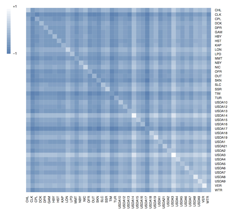
To account for population structure present in the data sets, we will estimate variance-covariance matrix of allele frequencies among populations. Ideally this inference should be drawn from variants that are (1) independent from the ones that would be tested for GENE x ENVIRONMENT correlation, and (2) reside in intronic regions of the genome unlikely to be under the action of natural selection.
We define these SNPs are intergenic, interpreted as such based on functional annotations. For this data set we have 1353 intergenic SNPs available for estimating this covariance matrix
ls -lh

-rw-r--r--@ 1 vikram   255K Oct 27 14:45 core336_ig.bayenv2
bayenv2 -i core336_ig.bayenv2 -p 42 -k 100000 -r 384729 > core336_matrix.out

tail -n 42 core_336_matrix.out > core336_final.matrix
Here we ran the 100K steps of MCMC to estimate the COVMAT. After every 5000 steps, a new matrix was generated. Thus, there were 200 matrices altogether. For further analysis we will only take the 200th matrix, which is what the tail command above does.
Use the following script to generate a covariance matrix heatmap.
### Load the gplots2 package
library(gplots)

## Load color brewer
library(RColorBrewer)

## Load SDMTools for legend.gradient
library(SDMTools)

## Insert column headers (pop names)
cat popnames 100kmatrix.out > 100kmatrix2.out


## First import the results.  The input is the output from the matrix_corr.r script (only if you are doing heatmap for correlations).  The code below is only for covariance matrix heatmap.  Add row names in the first column, convert spaces to tabs, save.
cov <- read.table('100kmatrix2.out', header=TRUE)

## apply labels from column 1 as row headers (names); Assuming that column 1 header is 'Variable'
row.names(cov) <- colnames(cov)

## We do not need the first row be treated as data, since it contains column labels. This example has 100 rows.
#cov <- cov[,2:19]

## Treat the data as matrix, just to be sure R treats it as matrix
#covmat <- as.matrix(cov)

## Check the dimensions to make sure you are getting what you wanted.  If your data has 10 rows 6 columns, it should say 10x6
dim(covmat)


## Heat Map begins

blue2white <- colorRampPalette(c('steelblue', 'white'))
#red2yellow <- colorRampPalette(c("red","yellow"))
#red2white <- colorRampPalette(c('red', 'white'))

## First create a pdf object
pdf(file='covmat_poplar.pdf', width=12, height=12)

heatmap.2(covmat,
symm=FALSE,
revC=FALSE,
Rowv=FALSE,
Colv=FALSE,
dendrogram= c("none"),  # replace none with column if you want dendrogram.
distfun = dist,
hclustfun = hclust,
xlab = '', ylab = '',
key=FALSE,
keysize=1,
trace="none",
density.info=c("none"),
margins=c(10,10),
#col=heat.colors(256),
#col=brewer.pal(9, 'YlOrRd')(20),
#col=red2yellow(20),
#colorRampPalette(brewer.pal(9,"YlOrRd"))(20),
#col=red2yellow(20),
col=blue2white(20),
cexRow=1, cexCol=1,
add.expr=TRUE
)

#points for the gradient legend
pnts = cbind(x=c(0.07,0.085,0.085,0.07), y=c(0.65,0.85,0.65,0.85))

#create the gradient legend
legend.gradient(pnts, blue2white(20), title=c(""), limits=c("-1","+1"), cex=0.9)


## Print it to pdf
dev.off()
For this exercise we are being provided with results from a principle component analysis with 18 bioclim variables in addition to latitude, longitude and elevation for each population. Of the 20 PCs obtained from this analysis, we will be using the top 3 principle components for further analysis.
ls -lh

-rw-r--r--@ 1 vikram  staff   5.8K Oct 27 21:21 core336.envPC


head core336.envPC

pop ind_code    PC1 PC2 PC3
CHL CHL_01  -3.40791108481855   -1.52091457948876   -1.16877641344633
CHL CHL_04  -3.56296514054725   -1.12029836620479   -1.39936931787457
CHL CHL_06  -3.416967588679 -1.53618443413472   -1.13292697567598
CHL CHL_07  -3.41698325358195   -1.53620836106472   -1.13291592456589
CHL CHL_08  -3.38206354781062   -1.5575548993799    -1.12343335695832
CHL CHL_12  -3.46186553649546   -1.4881034636552    -1.08729531518871
CHL CHL_13  -3.4428848885974    -1.52386887305361   -1.1035376179771
CLK CLK_01  2.77995425945649    0.247537146952795   -0.138362486476488
CLK CLK_02 2.71799500721176 0.309298083096405 -0.116937317422946Since the PCA data is currently at individual level, we need to aggregate it for populations.
df <- read.table('core336.envPC', header=T)

head(df)

  pop ind_code       PC1       PC2       PC3
1 CHL   CHL_01 -3.407911 -1.520915 -1.168776
2 CHL   CHL_04 -3.562965 -1.120298 -1.399369
3 CHL   CHL_06 -3.416968 -1.536184 -1.132927
4 CHL   CHL_07 -3.416983 -1.536208 -1.132916
5 CHL   CHL_08 -3.382064 -1.557555 -1.123433
6 CHL   CHL_12 -3.461866 -1.488103 -1.087295


df2.agr <- aggregate(df[,3:5], by=list(df$pop), FUN=mean)

head(df2.agr)

  Group.1        PC1        PC2        PC3
1     CHL -3.4416630 -1.4690190 -1.1640364
2     CLK  2.7714984  0.2861724 -0.1344567
3     CPL -1.1217782  0.3943519 -0.0594341
4     DCK  3.6059735  0.3551648  0.3055548
5     DPR -1.4359603 -1.6350937  0.1830463
6     GAM -0.0234029  1.4826197  2.6026243
write.table(df2.agr, "pc123.ENV.pop42", quote=F, sep='\t', row.names=F, col.names=T)
write.table(t(df2.agr), "pc123.ENV.tposed.pop42", quote=F, sep='\t', row.names=F, col.names=T)
df2.agr <- read.table('pc123.ENV.tposed.pop42', header=T)

head(df2.agr)

        CHL        CLK        CPL       DCK        DPR        GAM       HBY
1 -3.441663  2.7714984 -1.1217782 3.6059735 -1.4359603 -0.0234029 3.7067885
2 -1.469019  0.2861724  0.3943519 0.3551648 -1.6350937  1.4826197 0.4011548
3 -1.164036 -0.1344567 -0.0594341 0.3055548  0.1830463  2.6026243 0.3314839
         HST       KAP       LON        LPD        MMT        NBY        NIC
1 0.68821260 0.3395909 -4.428999 -3.0431315  2.9422146 -2.8078718 -1.1638967
2 0.61838209 0.5231060 -2.497800 -2.5955948 -0.8996871 -0.5479383 -3.3327755
3 0.01673952 0.2277868 -1.118786  0.2736758 -0.5324874  0.3210550  0.7223532
        OFR       OUT        SKN        SLC        SSR         TIM        TUR
1 3.8543355  3.527296  3.7102294 -3.0053015  0.2909058 -0.15395840  3.0278502
2 0.2837569 -1.309681 -0.9690802 -2.2857357 -5.0172599  0.07316681  0.4154857
3 0.2550614 -1.475017 -1.1126406  0.1827175 -5.5681024  0.28236407 -0.7913404
       USDA1     USDA10     USDA12     USDA13     USDA14     USDA15     USDA16
1  0.4190433 -0.1827119 -1.2563710 -0.6503396 -0.7170976 -2.5281129 -2.3997969
2 -2.2501734 -1.6839757 -1.3463352 -2.1405969 -2.9843278 -1.6951548 -1.7662754
3  2.4087908  1.5226147  0.1405484  0.4535536  0.5523843 -0.4934142 -0.8578083
      USDA17     USDA18     USDA19      USDA2    USDA21      USDA3      USDA4
1 -2.1383908 -2.0916993 -1.7176160  0.5126406 -0.921333 -0.6466922  0.7081282
2 -1.9344084 -2.8350151 -2.8041237 -2.0398049 -1.833369 -0.2643395 -1.0688186
3 -0.6445486 -0.7144912 -0.3402399  2.2239417  1.848250  1.2282314  1.9096496
       USDA5     USDA6     USDA7     USDA8     USDA9        VER        WTR
1  0.9008194  1.107652  1.226827  1.846822  1.665155 -3.4492268 -0.1898949
2 -1.1822345 -1.527163 -1.172686 -1.465682 -1.512212 -2.5426615  0.7077555
3  2.3122228  2.183572  2.149100  2.314840  2.273208  0.6722562  0.1320863
geno.poporder <- read.table('geno.poporder', header=F)

geno.poporder

       V1
1     CHL
2     CLK
3     CPL
4     DCK
5     DPR
6     GAM
7     HBY
8     HST
9     KAP
10    LON
11    LPD
12    MMT
13    NBY
14    NIC
15    OFR
16    OUT
17    SKN
18    SLC
19    SSR
20    TIM
21    TUR
22 USDA10
23 USDA12
24 USDA13
25 USDA14
26 USDA15
27 USDA16
28 USDA17
29 USDA18
30 USDA19
31  USDA1
32 USDA21
33  USDA2
34  USDA3
35  USDA4
36  USDA5
37  USDA6
38  USDA7
39  USDA8
40  USDA9
41    VER
42    WTR
df2.agr2 <- data.frame(df2.agr[,1:21], df2.agr[,23:31],df2.agr$USDA1,df2.agr$USDA21,df2.agr$USDA2,df2.agr[,34:42])

df2.agr2

        CHL        CLK        CPL       DCK        DPR        GAM       HBY
1 -3.441663  2.7714984 -1.1217782 3.6059735 -1.4359603 -0.0234029 3.7067885
2 -1.469019  0.2861724  0.3943519 0.3551648 -1.6350937  1.4826197 0.4011548
3 -1.164036 -0.1344567 -0.0594341 0.3055548  0.1830463  2.6026243 0.3314839
         HST       KAP       LON        LPD        MMT        NBY        NIC
1 0.68821260 0.3395909 -4.428999 -3.0431315  2.9422146 -2.8078718 -1.1638967
2 0.61838209 0.5231060 -2.497800 -2.5955948 -0.8996871 -0.5479383 -3.3327755
3 0.01673952 0.2277868 -1.118786  0.2736758 -0.5324874  0.3210550  0.7223532
        OFR       OUT        SKN        SLC        SSR         TIM        TUR
1 3.8543355  3.527296  3.7102294 -3.0053015  0.2909058 -0.15395840  3.0278502
2 0.2837569 -1.309681 -0.9690802 -2.2857357 -5.0172599  0.07316681  0.4154857
3 0.2550614 -1.475017 -1.1126406  0.1827175 -5.5681024  0.28236407 -0.7913404
      USDA10     USDA12     USDA13     USDA14     USDA15     USDA16     USDA17
1 -0.1827119 -1.2563710 -0.6503396 -0.7170976 -2.5281129 -2.3997969 -2.1383908
2 -1.6839757 -1.3463352 -2.1405969 -2.9843278 -1.6951548 -1.7662754 -1.9344084
3  1.5226147  0.1405484  0.4535536  0.5523843 -0.4934142 -0.8578083 -0.6445486
      USDA18     USDA19 df2.agr.USDA1 df2.agr.USDA21 df2.agr.USDA2      USDA3
1 -2.0916993 -1.7176160     0.4190433      -0.921333     0.5126406 -0.6466922
2 -2.8350151 -2.8041237    -2.2501734      -1.833369    -2.0398049 -0.2643395
3 -0.7144912 -0.3402399     2.4087908       1.848250     2.2239417  1.2282314
       USDA4      USDA5     USDA6     USDA7     USDA8     USDA9        VER
1  0.7081282  0.9008194  1.107652  1.226827  1.846822  1.665155 -3.4492268
2 -1.0688186 -1.1822345 -1.527163 -1.172686 -1.465682 -1.512212 -2.5426615
3  1.9096496  2.3122228  2.183572  2.149100  2.314840  2.273208  0.6722562
         WTR
1 -0.1898949
2  0.7077555
3  0.1320863
write.table(df2.agr2, 'pc123.ENV.pop42.Final', quote=F, sep='\t', row.names=F, col.names=T)At this point, we should have three pieces of information to perform environmental correlation using BAYENV2:
We will using allelic counts from CHR 3 only. The data is located in chr3_in folder:
ls chr3_in | head

S3_10169495
S3_10230391
S3_10288107
S3_10311268
S3_10420906
S3_10421038
S3_10421074
S3_10441317
S3_10441323
S3_10535587

ls chr3_in | wc -l

6388
runBayeChr3.sh ScriptThis script will run Bayenv2 on each SNP file and aggregate results into their own folders. Bayenv2 outputs three types of results:
### Shortcuts
covmat="./covmat"
envmat="./pc123.ENV.pop42.Final"
chr3_in="./chr3_in"
chr3_out="./chr3_out"

cd $chr1_in
echo "$(pwd)"

for snp in S*
do
  echo "Current time is $(date)"
  echo "Working on SNP: $snp"
  rnum="$(shuf -i 100000-900000 -n 1)"
  echo "Random Number: $rnum"
  bayenv2 -i $snp -m $covmat -e $envmat -p 42 -k 100000 -r $rnum -t -n 3 -f -X -o $chr3_out/core336_bayenv_chr3
  echo "Finished working on $snp at $(date)"
  echo ""
  echo "------------------------------------------"
  echo ""
done

mkdir $chr3_out/std.freqs
mkdir $chr3_out/bf
mkdir $chr3_out/xtx

mv $chr3_in/*.freqs $chr3_out/std.freqs/
echo "Standardized Allele Frequency Files for CHR3 are in:"
echo "${chr3_out}/std.freqs"

mv $chr3_out/*.bf $chr3_out/bf/
echo "Bayes Factors for CHR3 are in:"
echo "${chr3_out}/bf"

mv $chr3_out/*.xtx $chr3_out/xtx/
echo "XTX for CHR3 are in:"
echo "${chr3_out}/xtx"
Once the script finishes running, you should have 6387 individual output files each containing 3 Bayes Factors (and similarly separate files for standardized allele frequency and XTX components. First merge all the BF files together into a single file:
cd chr3_out

ls | wc -l

6387

cat *.bf > bf/core336_bayenv_chr3.bf

head core336_bayenv_chr3.bf

S3_1002415  1.7076e-01  3.2641e-01  1.7951e-01
S3_1002421  3.8559e+01  1.6463e+00  1.9971e-01
S3_1002437  4.6188e-01  3.7350e-01  3.3666e-01
S3_10054178 1.3006e-01  2.0003e-01  2.2075e-01
S3_10054179 1.8279e-01  2.5539e-01  2.4947e-01
S3_10054181 2.7824e-01  5.6616e-01  3.4301e-01
S3_101579   1.1257e-01  5.2501e-01  3.7978e-01
S3_101615   2.3428e-01  2.7866e-01  2.4620e-01
S3_10169455 2.9605e-01  2.5993e-01  2.0779e-01
S3_10169481 2.8951e-01  2.1797e-01  1.8969e-01
These are the Bayes Factors for each of the three PCs we analyzed, listed per tested SNP.
Bayenv tests every SNP under consideration for correlation against provided environmental variables. In our case, the envars are PC1, PC2 and PC3. Higher bayes factors indicate stronger correlation than lower. We will look at sites that are among the top 1% (highest bayes factors) for each of the PCs.
setwd("chr3_out/bf/")

bf336 <- read.table("core336_bayenv_chr3.bf", header=F)

head(bf336)

colnames(bf336) <- c("CHR_POS", "BF_PC1", "BF_PC2", "BF_PC3")

head(bf336)

      CHR_POS   BF_PC1  BF_PC2  BF_PC3
1  S3_1002415  0.17076 0.32641 0.17951
2  S3_1002421 38.55900 1.64630 0.19971
3  S3_1002437  0.46188 0.37350 0.33666
4 S3_10054178  0.13006 0.20003 0.22075
5 S3_10054179  0.18279 0.25539 0.24947
6 S3_10054181  0.27824 0.56616 0.34301


quantile(bf336$BF_PC1)
         0%         25%         50%         75%        100%
9.86880e-02 1.63280e-01 2.09790e-01 3.13995e-01 8.75500e+21


quantile(bf336$BF_PC2)
         0%         25%         50%         75%        100%
1.60630e-01 2.61165e-01 3.23830e-01 4.51890e-01 9.20010e+11


quantile(bf336$BF_PC3)
        0%        25%        50%        75%       100%
  0.140750   0.221445   0.266620   0.352180 234.600000
It appears that for all 3 PCs, the top candidate sites have orders of magnitude higher bayes factors.
We will make a simple scatterplots (one per PC) so as to visually identify extreme candidate outliers among a large pool of SNPs.
library(scales)

head(bf336)

      CHR_POS   BF_PC1  BF_PC2  BF_PC3
1  S3_1002415  0.17076 0.32641 0.17951
2  S3_1002421 38.55900 1.64630 0.19971
3  S3_1002437  0.46188 0.37350 0.33666
4 S3_10054178  0.13006 0.20003 0.22075
5 S3_10054179  0.18279 0.25539 0.24947
6 S3_10054181  0.27824 0.56616 0.34301


dim(bf336)

[1] 6387    4


pdf('bf336.pdf', width=11, height=4)
par(mfrow=c(1,3), mar=c(4,4,3,2)+0.1, oma=c(1,1,1,1)+0.1)

plot(c(1:6387), bf336$BF_PC1, pch=16, col=alpha('darkgreen', 0.7), cex=1, xlab='SNPs on CHR3', ylab='BF (PC1)')
legend('topleft', 'BF - PC1', cex=1.2)
plot(c(1:6387), bf336$BF_PC2, pch=16, col=alpha('darkgreen', 0.7), cex=1, xlab='SNPs on CHR3', ylab='BF (PC2)')
legend('topleft', 'BF - PC2', cex=1.2)
plot(c(1:6387), bf336$BF_PC3, pch=16, col=alpha('darkgreen', 0.7), cex=1, xlab='SNPs on CHR3', ylab='BF (PC3)')
legend('topleft', 'BF - PC3', cex=1.2)

title(main="BAYENV2 BF Indicating Selection Candidate SNPs", outer=TRUE, font.main=1, line=-1, cex.main=1.5)

dev.off()
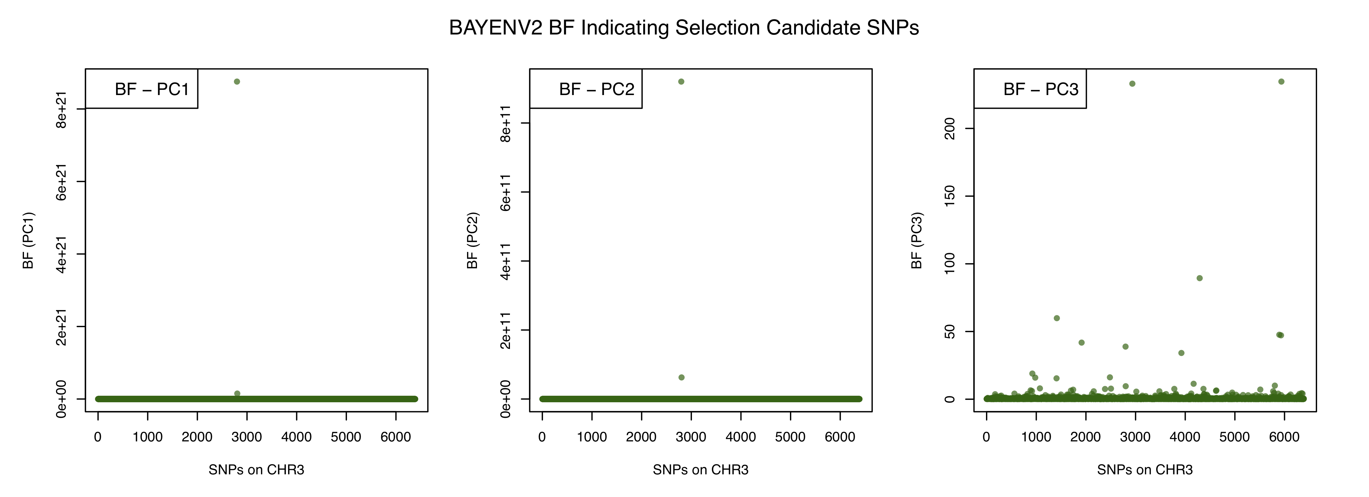
We can use the subset function in R to quickly identify the outliers for each PCs.
subset(bf336, BF_PC1 > 8e+21 | BF_PC2 > 8e+11 | BF_PC3 > 200)

         CHR_POS     BF_PC1     BF_PC2  BF_PC3
2798 S3_18489700 8.7550e+21 9.2001e+11  38.852
2935  S3_1891169 1.5174e-01 2.2109e+00 233.050
5937  S3_8437952 1.0663e+00 2.9591e-01 234.600
We were expecting four SNPs, but only found 3. If you look carefully, you will notice that the SNP S3_18489700 is an outlier for both PC1 and PC2. This indicates it is highly correlated to multiple environmental variables that are part of either PC1 or PC2. You can further investigate this by looking at genome annotations in P. trichocarpa to discern what functional pathways this SNP (and the other two) is involved in.